Notebook source code:
examples/geometry2D/ellipsoid/ellipsoid.ipynb
Run the notebook yourself on binder
![]()
The ellipsoid of revolution
by O. Cots, January 2022.
Abstract. In this notebook, we present how we can use numerical continuation methods (or homotopy) to compute the conjugate and cut loci of a 2-dimensional Riemannian manifold. These methods are applied to the case of an oblate ellipsoid of revolution.
Preliminary remarks. All the numerical experiments are computed with the nutopy package: see the documentation and the gallery of examples. See [Bonnard et al. 2014] for a previous work about geometric and numerical techniques (see the hampath software) to compute conjugate and cut loci on Riemannian surfaces. The main difference with the present
work is that in this notebook, we combine second order optimality computations with homotopy methods.
List of numerical algorithms to compute cut loci on a Riemannian manifold.
Preliminaries
We recall standard notions of Riemannian geometry [do Carmo 1988] [Berger 2003]. On a connected Riemannian manifold \((M, g)\) of dimension \(n\), the metric \(g\) induces a distance function \(d(q_0, q_1)\) for any pair \((q_0, q_1) \in M^2\). The distance \(d(q_0, q_1)\) being the infimum of lengths of continuously differentiable curves \(q\) joining the points \(q_0\) and \(q_1\). If we denote by \(l(q)\) the length of a curve \(q\), then on a connected and complete Riemannian manifold, for any pair \((q_0, q_1) \in M^2\), there exists a continuously differentiable curve \(q\) such that \(d(q_0, q_1) = l(q)\). In this case, the solution curve \(q\) being necessarily chosen among the set of the so-called geodesic curves (or geodesics). The geodesics are so candidates as minimizers and we know that every geodesic is a minimizing curve at least on short distances.
Our main goal is to compute for a fixed \(q_0 \in M\), the partial distance function \(d(q_0, \cdot)\) together with the set of minimizing geodesics, that is we want to find for any other point \(q_1 \in M\), the distance \(d(q_0, q_1)\) and the geodesics \(q\) such that \(d(q_0, q_1) = l(q)\). To do so, we have to compute the geodesics which are projections of extremals given by the flow of the Hamiltonian vector field \(\vec{H}\) associated to the Hamiltonian \(H\) given by the Legendre transform of the metric \(g\).
The cut point of a geodesic is the point where it ceases to be minimizing. Fixing \(q_0 \in M\), the set of cut points of all the geodesics starting from \(q_0\) is the cut locus denoted \(\mathrm{Cut}(q_0)\). Our main goal is thus equivalent to compute \(\mathrm{Cut}(q_0)\). We do so in the academic case of an oblate ellipsoid of revolution to illustrate the numerical tools. The theoretical results related to this case may be found in [Itoh-Kiohara 2004]. In the Riemannian frame, the cut points may be of two kinds, either conjugate points or isochronous separating points. A conjugate point is a point where the geodesic \(q\) ceases to be optimal among the geodesics \(C^1\)-close to \(q\). The conjugate points are fold points of the geodesic flow and are due to the intrinsic curvature of the Riemannian manifold. This points may be computed by linearization of the flow of \(\vec{H}\), that is computing Jacobi fields. An isochronous separating point is a point where two distincts minimizing geodesics intersect, that is it is a self-intersection of a wavefront of the geodesic flow. The set of separating points is called the separating locus.
Summary of the main goal
Our main goal is to compute the distance together with the minimizing geodesics, to do so, we aim to compute the cut locus which is made of conjugate points and isochronous separating points.
In Section 2 (Hamiltonian), we define the only one fundamental object for our computations, that is the Hamiltonian \(H\), in the case of an oblate ellipsoid of revolution. From the Hamiltonian, we define the Hamiltonian vector field \(\vec{H}\) and its flow. In Section 3 (Geodesics), we define the geodesic flow parameterized by the initial angle of the covector. The geodesics being parameterized by arc length, setting \(H = 1/2\). In Section 4 (Conjugate locus), we compute by differential continuation method (or homotopy) the set of first conjugate points, that is the conjugate locus. In Section 5 (Wavefronts), we compute self-intersections of wavefronts. Finally, in Section 6 (Cut locus), we compute the cut locus which is composed of two conjugate points and the separating locus, which is also computed by homotopy.
[1]:
# Packages
import numpy as np # scientific computing tools
import nutopy as nt # control toolbox: indirect methods and homotopy
import wrappers # for compilation of Fortran Hamiltonian codes
import plottings # for plots
import bdd # for saving data
Hamiltonian and flow
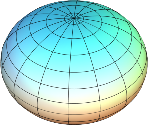
The Cartesian equation of the normalized 2-dimensional ellipsoid of revolution may be written as
The associated ellipsoid of revolution may be generated by a rotation of axis \(Oz\) of the parameterized curve
with \(u \in [0, 2\pi]\) and where \(0<\varepsilon<1\) corresponds to the oblate (flattened) case while \(\varepsilon >1\) is the prolate (elongated) case. The Cartesian coordinates may be parameterized by the azimuth \(\theta \in [-\pi, \pi]\) and the latitude \(\varphi \in [-\pi/2, \pi/2]\), by the relations
The restriction of the Euclidean metric of the ambient space \(\mathrm{R}^3\) gives the following induced metric on the ellipsoid:
where \(g_{1}(\varphi)=\cos^{2}\varphi\) and \(g_{2}(\varphi)=\sin^{2}\varphi+\varepsilon^{2}\cos^{2}\varphi\). In the following, we consider the oblate case and we fix \(\varepsilon = 0.75\) and \(q_0 = (0, 0)\). The Legendre transform of the metric \(g\) gives the associated Hamiltonian
From the Hamiltonian \(H\), we define the Hamiltonian vector field defined on the cotangent bundle \(T^*M\) (\(M\) being the ellipsoid)
We finally define the Hamiltonian exponential map, \(e^{t \vec{H}} \colon T^*M \to T^*M\), by
where the extremal \(z(\cdot, q_0, p_0)\) is defined as the maximal solution of the Cauchy problem \(\dot{z}(t) = \vec{H}(z(t))\), \(z(0) = (q_0, p_0)\). Thus, the Hamiltonian exponential map gives us the flow of extremals, associated to the Hamiltonian system.
[2]:
# Fortran Hamiltonian code
#
# We use Fortran code for performances and because we need to compute the derivatives
# of the Hamiltonian up to order 3, which is done by automatic differentiation,
# thanks to tapenade (https://team.inria.fr/ecuador/fr/tapenade/) software.
!pygmentize hfun.f90
subroutine hfun(x, p, epsi, h)
double precision, intent(in) :: x(2), p(2), epsi
double precision, intent(out) :: h
! local variables
double precision :: theta, phi, ptheta, pphi, g1, g2
theta = x(1)
phi = x(2)
ptheta = p(1)
pphi = p(2)
g1 = cos(phi)**2
g2 = sin(phi)**2+epsi**2*cos(phi)**2
h = 0.5d0 * (ptheta**2 / g1 + pphi**2 / g2)
end subroutine hfun
[3]:
# Parameters
epsilon = 0.75 # oblate case (epsilon < 1)
theta0 = 0.0 # initial azimuth
phi0 = 0.0 # initial latitude
t0 = 0.0 # initial time
# Initialize data
data_file = 'data.json'
restart = True # restart or not the computations
data = bdd.Data({'t0': t0, 'theta0': theta0, 'phi0': phi0, 'epsilon': epsilon}, data_file, restart)
# Initial point
q0 = np.array([theta0, phi0])
Initiate done
[4]:
h = wrappers.hamiltonian(epsilon, compile=True, display=False) # Hamiltonian and derivatives up to order 3
extremal = nt.ocp.Flow(h) # Hamiltonian exponential map and its derivatives: extremals and linearizations
Geodesics
By homogeneity, the extremals may be parameterized fixing \(H=1/2\). This amounts to parameterize the geodesics by the arc length. Thus, given an initial point \(q_0 \in M\), the initial covector \(p_0\) must satisfy \(H(q_0, p_0)=1/2\). One can write that \(p_0 \in S^1 = \{p ~|~ ||p||=1\}\), defining the norm \(||p||^2=2H(q_0,p)\) on \(T_{q_0}^*M\). Hence, the initial covector may be parameterized by its angle \(\alpha_0 \in [0,2\pi)\). We write
this parameterization. Finally, a geodesic starting from \(q_0\) is the projection of an extremal parameterized by its initial angle \(\alpha_0\) and is given by the following classical exponential map:
where \(\pi_q(q, p) = q\) is the canonical projection on the state space.
[5]:
# The Riemannian metric of the ellipsoid of revolution
# We get the metric from the Hamiltonian description
def metric(q):
h1 = h(t0, q, np.array([1.0, 0.0]))
h2 = h(t0, q, np.array([0.0, 1.0]))
g1 = 1.0/(2.0*h1)
g2 = 1.0/(2.0*h2)
return g1, g2
# Initial covector parameterization and its derivatives up to order 2
def covector(q, alpha):
g1, g2 = metric(q)
p0 = np.array([np.cos(alpha)*np.sqrt(g1),
np.sin(alpha)*np.sqrt(g2)])
return p0
def dcovector(q, alpha, dalpha):
g1, g2 = metric(q)
dp0 = np.array([-np.sin(alpha)*np.sqrt(g1)*dalpha,
np.cos(alpha)*np.sqrt(g2)*dalpha])
return dp0
def d2covector(q, alpha, dalpha, d2alpha):
g1, g2 = metric(q)
d2p0 = np.array([-np.cos(alpha)*np.sqrt(g1)*dalpha*d2alpha,
-np.sin(alpha)*np.sqrt(g2)*dalpha*d2alpha])
return d2p0
covector = nt.tools.tensorize(dcovector, d2covector, tvars=(2,))(covector)
[6]:
# Compute a geodesic parameterized by alpha0 to time t
# The initial point is fixed to q0 and t0 = 0
def tspan(t0, t):
N = 100
return list(np.linspace(t0, t, N+1))
def geodesic(t, alpha0):
p0 = covector(q0, alpha0)
q, p = extremal(t0, q0, p0, tspan(t0, t))
return q
# Function to plot geodesics
geodesics_plot = plottings.Geodesics(geodesic, epsilon)
[7]:
geodesics_plot.interact(embed=True)
[7]:
Conjugate locus
A point \(q(t_c)\) on an extremal \(z=(q,p)\) is conjugate to \(q_0 = q(0)\) if there exists a Jacobi field \(\delta z = (\delta q, \delta p)\), solution of the linearized system along the extremal,
which is non-trivial (\(\delta q \not \equiv 0\)) and vertical at \(t=0\) and \(t_c>0\) (called the conjugate time), that is \(\delta q(0) = \delta q(t_c) = 0\). The conjugate locus is the set of such first points on extremals departing from \(q_0\). Conjugacy is classicaly related to local optimality of extremals in the relevant topologies. Let \(q \colon t \mapsto \exp_{q_0}(t, \alpha_0)\) being a reference geodesic and introduce \(F_\mathrm{conj} \colon \mathrm{R}^*_+ \times [0, 2\pi) \to \mathrm{R}\) as
Then, in the Riemannian setting, \(q(t_c)\) is conjugate to \(q_0\) if and only if \(F_\mathrm{conj}(t_c, \alpha_0) = 0\). The conjugate locus from \(q_0\) is thus given by
where \(t_{1c}\) has to be understood in the sense that it is the first conjugate time. To compute the conjugate locus, we need to compute the first conjugate times, that is to compute
Algorithm
We have to compute a subset of \(F_\mathrm{conj}^{-1}(\{0\})\). We use the numerical continuation method (or homotopy method) [Allgower-Georg 2003] implemented in the nutopy package. Under some regularity assumptions, the set \(F_\mathrm{conj}^{-1}(\{0\})\) is a disjoint union of differential curves, each curve being called a path of zeros. To compute a path of zeros, we search a first point on the curve by fixing the homotopic parameter (here it will be
\(\alpha_0\)) to a certain value \(\alpha_0^*\) and then calling a Newton method to solve \(F_\mathrm{conj}(\cdot, \alpha_0^*) = 0\). The Newton solver in the nutopy package is the hybrj code from the minpack library [Moré et al. 1980].
When we have our initial point on the path of zeros, we use a Predictor-Corrector (PC) method with arc length parameterization to compute the differential curve. The nutopy package implements a PC method with a high-order Runge-Kutta scheme with adaptive step size for the prediction [Hairer et al. 1993], so we compute the path of zeros with high precision and we let the integration solver to construct the discretization
grid of the homotopic parameter. The prediction part is the same as in the hampath software [Caillau et al. 2011]. The correction step is performed by a simplified Newton algorithm [Hairer-Wanner 1996, page 119] with few iterations and where the Jacobian of the associated system to solve is not updated along the iterations.
For the prediction and the correction steps, we need to compute the Jacobian of \(F_\mathrm{conj}\). It is computed by a combination of automatic differentiation (to get \(\vec{H}\) and its derivatives up to order 2) performed with tapenade software [Hascoët-Pascual 2012] and variational equations to compute Jacobi fields and their derivatives with respect to the initial angle \(\alpha_0\).
[8]:
# Jacobi field: dz(t, p(alpha0), dp(alpha0))
@nt.tools.vectorize(vvars=(1,))
def jacobi(t, alpha0):
p0, dp0 = covector(q0, (alpha0, 1.))
(q, dq), (p, dp) = extremal(t0, q0, (p0, dp0), t)
return (q, dq), (p, dp)
# Derivative of dq w.r.t. t and alpha0
def djacobi(t, alpha0):
#
p0, dp0, d2p0 = covector(q0, (alpha0, 1., 1.))
#
(q, dq1, d2q), (p, dp1, _) = extremal(t0, q0, (p0, dp0, dp0), t)
(q, dq2), (p, dp2) = extremal(t0, q0, (p0, d2p0), t)
#
hv, dhv = h.vec(t, (q, dq1), (p, dp1))
#
ddqda = d2q+dq2 # ddq/dalpha
ddqdt = dhv[0:2] # ddq/dt
return (q, dq1), (p, dp1), (ddqdt, ddqda)
[9]:
# Function to compute conjugate time together with the initial angle
# and the associated conjugate point
#
# conjugate(tc, qc, a0) = ( det( dq(tc, a0), Hv(tc, z(tc, a0)) ),
# qc - pi_q(z(tc, a0)) ),
#
# where pi_q(q, p) = q and z(t, a) = extremal(t0, q0, p(a), t).
#
# Remark: y = (tc, qc)
#
def conjugate(y, a):
tc = y[0]
qc = y[1:3]
alpha0 = a[0]
#
(q, dq), (p, dp) = jacobi(tc, alpha0)
hv = h.vec(tc, q, p)[0:2]
#
c = np.zeros(3)
c[0] = np.linalg.det([hv, dq])
c[1:3] = qc - q
return c
# Derivative of conjugate
def dconjugate(y, a):
tc = y[0]
qc = y[1:3]
alpha0 = a[0]
#
(q, dq), (p, dp), (ddqdt, ddqda) = djacobi(tc, alpha0)
#
# dc/da
hv, dhv = h.vec(tc, (q, dq), (p, dp))
dcda = np.zeros((3, 1))
dcda[0,0] = np.linalg.det([dhv[0:2], dq])+np.linalg.det([hv[0:2], ddqda])
dcda[1:3,0] = -dq
#
# dc/dy = (dc/dt, dc/dq)
hv, dhv = h.vec(tc, (q, hv[0:2]), (p, hv[2:4]))
dcdy = np.zeros((3, 3))
dcdy[0,0] = np.linalg.det([dhv[0:2], dq])+np.linalg.det([hv[0:2], ddqdt])
dcdy[1:3,0] = -hv[0:2]
dcdy[1,1] = 1.
dcdy[2,2] = 1.
return dcdy, dcda
[10]:
def get_conjugate_locus():
# -------------------------
# Get first conjugate point
# Initial guess
gap = 1e-2
tci = np.pi
alpha = np.array([-np.pi/2+gap])
p0 = covector(q0, float(alpha))
xi, pi = extremal(t0, q0, p0, tci)
yi = np.zeros(3)
yi[0] = tci
yi[1:3] = xi
# Equations and derivative
fun = lambda t: conjugate(t, alpha)
dfun = lambda t: dconjugate(t, alpha)[0]
# Callback
def print_conjugate_time(infos):
print(' Conjugate time estimation: tc = %e for alpha = %e' % (infos.x[0], alpha), end='\r')
# Options
opt = nt.nle.Options(Display='on')
# Conjugate point calculation for initial homotopic parameter
print(' > Get first conjugate time and point:\n')
sol = nt.nle.solve(fun, yi, df=dfun, callback=print_conjugate_time, options=opt)
# -------------------
# Get conjugate locus
# Options
opt = nt.path.Options(MaxStepSizeHomPar=0.05, Display='on');
# Homotopic parameter range: we compute only half of the conjugate locus
# the other part is obtained by symmetry
alpha0 = alpha
alphaf = np.pi/2.-gap
# Initial solution
y0 = sol.x
# Callback
def progress(infos):
current = float(infos.pars)-alpha0
total = alphaf-alpha0
barLength = 50
percent = float(current * 100.0 / total)
arrow = '-' * int(percent/100 * barLength - 1) + '>'
spaces = ' ' * (barLength - len(arrow))
print(' Progress: [%s%s] %1.2f %%' % (arrow, spaces, round(percent, 2)), end='\r')
# Conjugate locus calculation
print('\n\n > Get conjugate locus:\n')
sol = nt.path.solve(conjugate, y0, alpha0, alphaf, options=opt, df=dconjugate) #, callback=progress)
print('\n')
return sol.xout
[11]:
# Get conjugate locus
if data.contains('conjugate_locus') and not restart:
conjugate_locus = np.array(data.get('conjugate_locus')); print('Conjugate locus loaded')
else:
conjugate_locus = get_conjugate_locus()
data.update({'conjugate_locus':conjugate_locus.tolist()}); print('Conjugate locus saved')
# Function to plot the conjugate locus
conjugate_plot = plottings.Conjugate_Locus(conjugate_locus, epsilon)
> Get first conjugate time and point:
Calls |f(x)| |x|
1 3.936995823975282e-01 4.467647749516624e+00
2 4.278155636398811e-02 4.672169273455422e+00ha = -1.560796e+00
3 4.722661649310230e-03 4.650876408102643e+00ha = -1.560796e+00
4 3.351515768332736e-05 4.652974457351447e+00ha = -1.560796e+00
5 4.566345728662711e-07 4.652989155900476e+00ha = -1.560796e+00
6 6.933441770142508e-09 4.652988953911271e+00ha = -1.560796e+00
7 6.032213481406154e-12 4.652988950795741e+00ha = -1.560796e+00
Conjugate time estimation: tc = 3.351569e+00 for alpha = -1.560796e+00
Results of the nle solver method:
xsol = [3.35156853 3.14159181 0.7400645 ]
f(xsol) = [-5.89486114e-12 -8.34887715e-14 1.27720057e-12]
nfev = 7
njev = 1
status = 1
success = True
Successfully completed: relative error between two consecutive iterates is at most TolX.
> Get conjugate locus:
Calls |f(x,pars)| |x| Homotopic param Arclength s det A(s) Dot product
1 3.36217081e-16 4.65298895079e+00 -1.56079632679e+00 0.00000000e+00 -2.10225656e+00 0.00000000e+00
2 5.77742394e-13 4.65283083245e+00 -1.55223936044e+00 8.56107018e-03 -2.10300750e+00 9.99832773e-01
3 5.84715180e-13 4.65228799944e+00 -1.53660176544e+00 2.42242662e-02 -2.10553835e+00 9.99443401e-01
4 7.74366996e-14 4.65032495696e+00 -1.50702697627e+00 5.39659520e-02 -2.11437003e+00 9.98033109e-01
5 2.10209079e-14 4.64452284645e+00 -1.46009822249e+00 1.01725692e-01 -2.13885089e+00 9.95225781e-01
6 3.95429722e-16 4.63442490080e+00 -1.41009822249e+00 1.53822109e-01 -2.17786443e+00 9.94965694e-01
6 6.55629916e-12 4.63052344604e+00 -1.39495252337e+00 1.69926644e-01 -2.17786443e+00 9.94965694e-01
7 2.62314084e-16 4.61473732598e+00 -1.34495252337e+00 2.24404281e-01 -2.24515108e+00 9.92513686e-01
7 3.69787613e-10 4.60685712041e+00 -1.32423756361e+00 2.47639686e-01 -2.24515108e+00 9.92513686e-01
8 1.10196606e-15 4.58452059946e+00 -1.27423756361e+00 3.05557633e-01 -2.33239968e+00 9.92870424e-01
8 1.30628830e-10 4.57198025255e+00 -1.24999003099e+00 3.34658131e-01 -2.33239968e+00 9.92870424e-01
9 4.80644813e-16 4.54257820059e+00 -1.19999003099e+00 3.96931156e-01 -2.43025014e+00 9.94102156e-01
9 2.27122364e-11 4.52870510519e+00 -1.17883539796e+00 4.24240654e-01 -2.43025014e+00 9.94102156e-01
10 3.26545324e-16 4.49256405662e+00 -1.12883539796e+00 4.91157125e-01 -2.52107133e+00 9.96125663e-01
10 1.41916037e-11 4.47697946530e+00 -1.10904985207e+00 5.18574158e-01 -2.52107133e+00 9.96125663e-01
11 1.44051684e-16 4.43443170871e+00 -1.05904985207e+00 5.90256707e-01 -2.60055332e+00 9.97385979e-01
11 1.38531041e-11 4.41615748110e+00 -1.03903368375e+00 6.19915012e-01 -2.60055332e+00 9.97385979e-01
12 9.00468956e-17 4.36752408119e+00 -9.89033683753e-01 6.96371942e-01 -2.66597520e+00 9.98178838e-01
12 1.11933162e-11 4.34484215037e+00 -9.67053497959e-01 7.31032647e-01 -2.66597520e+00 9.98178838e-01
13 1.59663385e-16 4.29044172045e+00 -9.17053497959e-01 8.12169167e-01 -2.71466712e+00 9.98683996e-01
13 8.87178375e-12 4.26152038299e+00 -8.91765435103e-01 8.54361387e-01 -2.71466712e+00 9.98683996e-01
14 6.11328735e-16 4.20177049944e+00 -8.41765435103e-01 9.39890557e-01 -2.74211822e+00 9.99022494e-01
14 6.84569137e-12 4.16506343481e+00 -8.12277990008e-01 9.91525561e-01 -2.74211822e+00 9.99022494e-01
15 4.59628602e-16 4.10063443824e+00 -7.62277990008e-01 1.08080777e+00 -2.74107317e+00 9.99238774e-01
15 2.53598171e-12 4.05579607582e+00 -7.28520549530e-01 1.14209503e+00 -2.74107317e+00 9.99238774e-01
16 1.50373649e-16 3.98783318359e+00 -6.78520549530e-01 1.23391294e+00 -2.70141488e+00 9.99312873e-01
16 3.77405158e-12 3.93654088059e+00 -6.41411148461e-01 1.30250105e+00 -2.70141488e+00 9.99312873e-01
17 5.70033059e-16 3.86688402129e+00 -5.91411148461e-01 1.39488960e+00 -2.61242143e+00 9.99151101e-01
17 4.66747130e-12 3.81620674579e+00 -5.55004158048e-01 1.46170323e+00 -2.61242143e+00 9.99151101e-01
18 1.38940538e-16 3.74740098143e+00 -5.05004158048e-01 1.55212918e+00 -2.47233825e+00 9.98684418e-01
18 1.21855294e-12 3.72614170756e+00 -4.89315634020e-01 1.58005587e+00 -2.47233825e+00 9.98684418e-01
19 2.50057839e-16 3.65997685872e+00 -4.39315634020e-01 1.66718032e+00 -2.33187599e+00 9.98729410e-01
19 1.81254752e-12 3.65207762296e+00 -4.33193369808e-01 1.67762307e+00 -2.33187599e+00 9.98729410e-01
20 7.84874384e-16 3.59117371607e+00 -3.84445674940e-01 1.75871308e+00 -2.19457718e+00 9.98625018e-01
21 1.16016696e-15 3.54086839454e+00 -3.41357577646e-01 1.82697003e+00 -2.07650992e+00 9.98766677e-01
22 1.33453408e-15 3.49915191638e+00 -3.02691869545e-01 1.88516005e+00 -1.96520489e+00 9.98622707e-01
23 1.91116368e-15 3.46440245247e+00 -2.67471198096e-01 1.93547554e+00 -1.86159075e+00 9.98448019e-01
24 5.22445396e-16 3.43245589811e+00 -2.31467781133e-01 1.98418043e+00 -1.75602853e+00 9.97806297e-01
25 1.55933646e-15 3.40604611640e+00 -1.97657553185e-01 2.02741557e+00 -1.65995527e+00 9.97394802e-01
26 1.70599868e-15 3.38425814214e+00 -1.65290125315e-01 2.06661846e+00 -1.57360520e+00 9.96850879e-01
27 5.64633118e-17 3.36664567448e+00 -1.34036425052e-01 2.10258991e+00 -1.49831689e+00 9.96219777e-01
28 4.57610102e-16 3.35240967335e+00 -1.02438470058e-01 2.13729718e+00 -1.43331244e+00 9.95155254e-01
29 1.82964717e-15 3.34210940178e+00 -7.16657098651e-02 2.16977429e+00 -1.38364908e+00 9.94444267e-01
30 7.88965034e-16 3.33617700593e+00 -4.54805550564e-02 2.19663541e+00 -1.35393633e+00 9.95402636e-01
31 7.07375853e-17 3.33292560626e+00 -1.98205498465e-02 2.22251113e+00 -1.33728275e+00 9.95218862e-01
32 5.67289216e-16 3.33219350111e+00 4.01312224174e-03 2.24636455e+00 -1.33349558e+00 9.95727846e-01
33 5.69372621e-16 3.33352498588e+00 2.64849308369e-02 2.26888288e+00 -1.34037302e+00 9.96223509e-01
34 5.28997031e-16 3.33678438236e+00 4.88050525766e-02 2.29144678e+00 -1.35701778e+00 9.96423325e-01
35 1.66947380e-15 3.34211508798e+00 7.16862645022e-02 2.31494958e+00 -1.38367716e+00 9.96510538e-01
36 6.30365696e-16 3.34983204654e+00 9.56508988420e-02 2.34014070e+00 -1.42110290e+00 9.96565863e-01
37 2.39890791e-15 3.36077349326e+00 1.21959163489e-01 2.36866417e+00 -1.47198451e+00 9.96425954e-01
38 5.52061780e-16 3.37828603309e+00 1.55353615342e-01 2.40645602e+00 -1.54866626e+00 9.95313888e-01
39 1.06248862e-15 3.39778614853e+00 1.85988510549e-01 2.44291366e+00 -1.62803471e+00 9.96920072e-01
40 1.23730409e-15 3.41916995400e+00 2.15036688685e-01 2.47921164e+00 -1.70878480e+00 9.97834829e-01
41 2.57517180e-15 3.44303786314e+00 2.43877850653e-01 2.51699742e+00 -1.79219613e+00 9.98330374e-01
42 1.04724911e-15 3.46981667094e+00 2.73188101615e-01 2.55721552e+00 -1.87845571e+00 9.98654678e-01
43 1.07548426e-15 3.50013832931e+00 3.03646149909e-01 2.60094198e+00 -1.96799327e+00 9.98871713e-01
44 1.08113343e-15 3.53466766725e+00 3.35806922017e-01 2.64919504e+00 -2.06078575e+00 9.99029444e-01
45 1.51719842e-15 3.57418040225e+00 3.70236659686e-01 2.70310315e+00 -2.15650514e+00 9.99149143e-01
46 1.40745439e-15 3.61955004831e+00 4.07534031825e-01 2.76392073e+00 -2.25434537e+00 9.99244595e-01
47 1.66778075e-15 3.67177076663e+00 4.48387076033e-01 2.83309210e+00 -2.35291509e+00 9.99324010e-01
48 9.98599896e-16 3.73194506621e+00 4.93612941474e-01 2.91227133e+00 -2.45001350e+00 9.99393033e-01
49 2.01048489e-16 3.80042294229e+00 5.43612941474e-01 3.00223675e+00 -2.54137311e+00 9.99465904e-01
49 8.59699028e-14 3.80128195501e+00 5.44233827455e-01 3.00336630e+00 -2.54137311e+00 9.99465904e-01
50 1.17826554e-16 3.87082079240e+00 5.94233827455e-01 3.09501534e+00 -2.61611734e+00 9.99602147e-01
50 1.35606344e-12 3.88096499022e+00 6.01506565208e-01 3.10843018e+00 -2.61611734e+00 9.99602147e-01
51 4.75742083e-16 3.95054629753e+00 6.51506565208e-01 3.20087675e+00 -2.67926744e+00 9.99614698e-01
51 1.91926025e-12 3.97192024909e+00 6.66963967585e-01 3.22945227e+00 -2.67926744e+00 9.99614698e-01
52 1.33372867e-16 4.04023538910e+00 7.16963967585e-01 3.32147842e+00 -2.72488759e+00 9.99576808e-01
52 1.61160577e-12 4.07404137602e+00 7.42169640568e-01 3.36747094e+00 -2.72488759e+00 9.99576808e-01
53 5.64454588e-16 4.13946386345e+00 7.92169640568e-01 3.45751274e+00 -2.74536964e+00 9.99415300e-01
53 4.21965273e-12 4.18442298114e+00 8.27726876347e-01 3.52033237e+00 -2.74536964e+00 9.99415300e-01
54 4.29729479e-17 4.24507866673e+00 8.77726876347e-01 3.60660080e+00 -2.73221579e+00 9.98983514e-01
54 1.07032852e-11 4.29578645734e+00 9.21816899287e-01 3.68039616e+00 -2.73221579e+00 9.98983514e-01
55 1.61817654e-16 4.34982324419e+00 9.71816899287e-01 3.76123467e+00 -2.67945262e+00 9.98063478e-01
55 2.80432977e-11 4.39829638798e+00 1.02016290030e+00 3.83632657e+00 -2.67945262e+00 9.98063478e-01
56 3.12232205e-16 4.44427459354e+00 1.07016290030e+00 3.91067519e+00 -2.58874713e+00 9.96459022e-01
56 3.58128429e-11 4.47375387033e+00 1.10506499383e+00 3.96054157e+00 -2.58874713e+00 9.96459022e-01
57 5.48533528e-16 4.51210725427e+00 1.15506499383e+00 4.02906912e+00 -2.48842282e+00 9.95738990e-01
57 1.85351298e-11 4.53251580448e+00 1.18451907649e+00 4.06785685e+00 -2.48842282e+00 9.95738990e-01
58 7.34614025e-16 4.56339256750e+00 1.23451907649e+00 4.13110903e+00 -2.38459058e+00 9.94417320e-01
58 1.57446508e-10 4.58140126273e+00 1.26799906949e+00 4.17172367e+00 -2.38459058e+00 9.94417320e-01
59 6.09843207e-16 4.60432733985e+00 1.31799906949e+00 4.22998168e+00 -2.27712077e+00 9.91240521e-01
59 3.85307694e-10 4.61612211201e+00 1.34882433425e+00 4.26459538e+00 -2.27712077e+00 9.91240521e-01
60 4.84023117e-16 4.63155904485e+00 1.39882433425e+00 4.31890889e+00 -2.18830430e+00 9.89099925e-01
60 1.15124381e-09 4.63883737408e+00 1.42947533172e+00 4.35125080e+00 -2.18830430e+00 9.89099925e-01
61 4.85400046e-16 4.64733335647e+00 1.47947533172e+00 4.40280386e+00 -2.12723441e+00 9.86868814e-01
61 4.54871888e-11 4.65069994450e+00 1.51146292969e+00 4.43521088e+00 -2.12723441e+00 9.86868814e-01
62 3.87323870e-16 4.65298895079e+00 1.56079632679e+00 4.48470255e+00 -2.10225656e+00 9.85263608e-01
Results of the path solver method:
xf = [ 3.35156853 3.14159181 -0.7400645 ]
parsf = [1.56079633]
|f(xf,parsf)| = 3.87323869939913e-16
steps = 89
status = 1
success = True
Homotopy successfully completed.
Update done
Conjugate locus saved
[12]:
# Plots on the 2D chart
fig = geodesics_plot(nb_geodesics=5) # Plot geodesics
conjugate_plot(fig=fig) # Plot conjugate locus
[12]:
<Figure size 675x720 with 1 Axes>
[ ]:
# Plots on the Ellipsoid
fig = geodesics_plot(coords=plottings.Coords.ELLIPSOID, nb_geodesics=5) # Plot geodesics
conjugate_plot(coords=plottings.Coords.ELLIPSOID, fig=fig) # Plot conjugate locus
Figures
Geodesics departing from \(q_0=(0,0)\) for different \(\alpha_0 \in [0, 2\pi)\). Note the envelope when the flow of the geodesics is folding. This is the conjugate locus (in red).
Wavefronts
The wavefront at time \(t \ge 0\) departing from \(q_0 \in M\) is given by
To emphasize the numerical methodology that we use to compute the wavefront, we define
Fixing \(q_0 \in M\) and \(t\ge 0\) and introducing \(F_\mathrm{front}\colon M^2 \times [0,2\pi) \to \mathrm{R}^2\) by
then we have \(\mathrm{Front}(q_0, t) = F_\mathrm{front}^{-1}(\{0\})\). Hence, \(F_\mathrm{front}\) is an homotopic function and \(\mathrm{Front}(q_0, t)\) is a path of zeros of \(F_\mathrm{front}\) that can be computed by differential homotopy methods. Once we have computed a wavefront, we compute a self-intersection of it, if any, to get our first cut point which is used in the following to compute the cut locus.
[ ]:
# Equation to calculate wavefronts
def wavefront_eq(q, alpha0, tf):
p0 = covector(q0, float(alpha0))
qf, _ = extremal(t0, q0, p0, tf)
return q - qf
# Derivative
def dwavefront_eq(q, dq, alpha0, dalpha0, tf):
p0, dp0 = covector(q0, (float(alpha0), float(dalpha0)))
(qf, dqf), _ = extremal(t0, q0, (p0, dp0), tf)
return q-qf, dq - dqf
wavefront_eq = nt.tools.tensorize(dwavefront_eq, tvars=(1, 2), full=True)(wavefront_eq)
[ ]:
# Function to compute wavefront at time tf, q0 being fixed
def get_wavefront(tf):
# Options
opt = nt.path.Options(Display='off', MaxStepSizeHomPar=0.1, MaxIterCorrection=0);
# Homotopic parameter range
epsi = 1e-4
alpha0 = -np.pi/2.0+epsi
alphaf = np.pi/2.0-epsi
# Initial solution
p0 = covector(q0, alpha0)
xf0, _ = extremal(t0, q0, p0, tf)
# callback
def progress(infos):
current = float(infos.pars)-alpha0
total = alphaf-alpha0
barLength = 50
percent = float(current * 100.0 / total)
arrow = '-' * int(percent/100.0 * barLength - 1) + '>'
spaces = ' ' * (barLength - len(arrow))
print(' Progress: [%s%s] %1.2f %%' % (arrow, spaces, round(percent, 2)), end='\r')
# wavefront computation
print('\n > Get wavefront for tf =', tf, '\n')
sol = nt.path.solve(wavefront_eq, xf0, alpha0, alphaf, args=tf, options=opt, df=wavefront_eq, callback=progress)
print('\n')
wavefront = (sol.xout, sol.parsout, tf)
return wavefront
[ ]:
# Get wavefronts
if data.contains('wavefronts') and not restart:
wavefronts = data.get('wavefronts'); print('Wavefronts loaded')
else:
wavefronts = []
wavefront = get_wavefront(tf=2.7);
wavefronts.append((wavefront[0].tolist(), wavefront[1].tolist(), wavefront[2]))
data.update({'wavefronts':wavefronts}); print('wavefronts saved')
# Function to plot wavefronts
wavefronts_plot = plottings.Wavefronts(wavefronts, epsilon)
[ ]:
# Plots on the 2D chart
fig = geodesics_plot(nb_geodesics=5, tf=2.7) # geodesics
conjugate_plot(fig=fig) # conjugate locus
wavefronts_plot(fig=fig) # wavefronts
[ ]:
# Plots on the Ellipsoid
fig = geodesics_plot(coords=plottings.Coords.ELLIPSOID, nb_geodesics=7, tf=2.7) # geodesics
conjugate_plot(coords=plottings.Coords.ELLIPSOID, fig=fig) # conjugate locus
wavefronts_plot(coords=plottings.Coords.ELLIPSOID, fig=fig) # wavefronts
Figures
Geodesics departing from \(q_0=(0,0)\) for different \(\alpha_0 \in [0, 2\pi)\) with \(t_f=2.7\). The conjugate locus is in red. The wavefront at time \(t_f = 2.7\) is represented in green. The self-intersections of the wavefront are isochronous separating points.
[ ]:
# Function to computes self-intersections of a curve in a 2-dimensional space
def get_self_intersections(curve):
n = curve[:,0].size
intersections = []
for i in range(n-3):
A = curve[i,:]
B = curve[i+1,:]
for j in range(i+2,n-1):
C = curve[j,:]
D = curve[j+1,:]
# Matrice M : M z = b
m11 = B[0] - A[0]
m12 = C[0] - D[0]
m21 = B[1] - A[1]
m22 = C[1] - D[1]
det = m11*m22-m12*m21
if(np.abs(det)>1e-8):
b1 = C[0] - A[0]
b2 = C[1] - A[1]
la = (m22*b1-m12*b2)/det
mu = (m11*b2-m21*b1)/det
if(la>=0. and la<=1. and mu>=0. and mu<=1.):
xx = {'i': i, 'j': j, 'x': np.array(A + la * (B-A)), 'la': la, 'mu': mu}
intersections.append(xx)
return intersections
[ ]:
# We compute one self-intersection of the wavefront
wa = wavefronts[0]
wavefront = np.array(wa[0])
alphas = np.array(wa[1])
tf = wa[2]
xxs = get_self_intersections(wavefront)
xx = xxs[0]
x = xx.get('x')
i = xx.get('i')
j = xx.get('j')
la = xx.get('la')
mu = xx.get('mu')
alpha1 = alphas[i]+la*(alphas[i+1]-alphas[i])
alpha2 = alphas[j]+mu*(alphas[j+1]-alphas[j])
print('Self-intersection of the wavefront for tf =', tf, 'at q = (', x[0], ',', x[1], ')\n')
print('alpha1 =', alpha1)
print('alpha2 = ', alpha2)
Cut locus
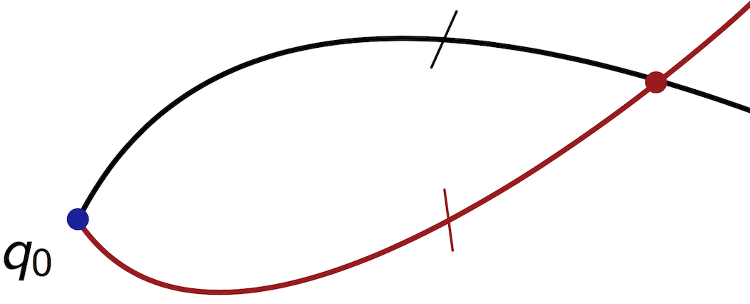
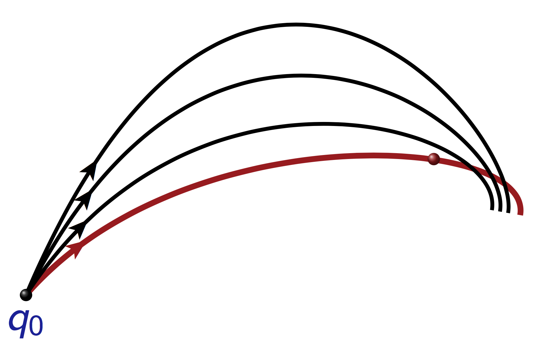
The cut locus \(\mathrm{Cut}(q_0)\) is the union of the cut points of the geodesics departing from \(q_0\). A cut point is either a conjugate point or an isochronous separating point [do Carmo 1988, page 267 Prop. 2.2], that is a point where two minimizing geodesics intersect with the same time (or length). A separating point (or splitting point) corresponds to a self-intersection of a wavefront. To compute the cut locus we need at this stage, to compute the separating locus (or splitting locus) and then compare for each geodesic its first conjugate time with its separating time. We introduce the following mapping:
The splitting locus is then given by solving \(F_\mathrm{split} = 0\) since we have
The splitting locus is also computed by homotopy. At the end, the cut locus of the oblate ellipsoid of revolution is the union of the splitting locus with the two conjugate points at the extremity of \(\mathrm{Split}(q_0)\) [Itoh-Kiohara 2004], that is
where \(t^*\) is by symmetry, the first positive time solution of
Note that \(t^*\) is the so-called injectivity radius.
|
|
Separating point | Conjugate point |
[ ]:
# Equations to compute Split(q0)
def split_eq(y, alpha2):
# y = (t, alpha1, q)
t = y[0]
a1 = y[1]
q = y[2:4]
a2 = float(alpha2)
q1, _ = extremal(t0, q0, covector(q0, a1), t)
q2, _ = extremal(t0, q0, covector(q0, a2), t)
eq = np.zeros(4)
eq[0:2] = q-q1
eq[2:4] = q-q2
return eq
# Derivative
def dsplit_eq(y, dy, alpha2, dalpha2):
t, dt = y[0], dy[0]
a1, da1 = y[1], dy[1]
q, dq = y[2:4], dy[2:4]
a2, da2 = float(alpha2), float(dalpha2)
(q1, dq1), _ = extremal(t0, q0, covector(q0, (a1, da1)), (t, dt))
(q2, dq2), _ = extremal(t0, q0, covector(q0, (a2, da2)), (t, dt))
eq, deq = np.zeros(4), np.zeros(4)
eq[0:2], deq[0:2] = q-q1, dq-dq1
eq[2:4], deq[2:4] = q-q2, dq-dq2
return eq, deq
split_eq = nt.tools.tensorize(dsplit_eq, tvars=(1, 2), full=True)(split_eq)
[ ]:
# Function to compute the splitting locus
def get_splitting_locus(q, a1, t, a2):
# Options
opt = nt.path.Options(MaxStepSizeHomPar=0.05, Display='off');
# Homotopic parameter range
epsi = 1e-3
alpha0 = 0.+epsi
alphaf = np.pi/2.0-epsi
# Initial solution
y0 = np.array([t, a1, q[0], q[1]])
b0 = a2
# callback
def progress_bis(infos):
current = b0-float(infos.pars)
total = alphaf-alpha0+b0-alpha0
barLength = 50
percent = float(current * 100.0 / total)
arrow = '-' * int(percent/100.0 * barLength - 1) + '>'
spaces = ' ' * (barLength - len(arrow))
print(' Progress: [%s%s] %1.2f %%' % (arrow, spaces, round(percent, 2)), end='\r')
# First homotopy
print('\n > Get splitting locus\n')
sol = nt.path.solve(split_eq, y0, b0, alpha0, options=opt, df=split_eq, callback=progress_bis)
ysol = sol.xf
# callback
def progress(infos):
current = b0-alpha0+float(infos.pars)-alpha0
total = alphaf-alpha0+b0-alpha0
barLength = 50
percent = float(current * 100.0 / total)
arrow = '-' * int(percent/100.0 * barLength - 1) + '>'
spaces = ' ' * (barLength - len(arrow))
print(' Progress: [%s%s] %1.2f %%' % (arrow, spaces, round(percent, 2)), end='\r')
# Splitting locus computation
sol = nt.path.solve(split_eq, ysol, alpha0, alphaf, options=opt, df=split_eq, callback=progress)
print('\n')
splitting_locus = sol.xout
return splitting_locus
[ ]:
# Get splitting locus
if data.contains('splitting_locus') and not restart:
splitting_locus = np.array(data.get('splitting_locus')); print('Splitting locus loaded')
else:
splitting_locus = get_splitting_locus(x, alpha1, tf, alpha2)
data.update({'splitting_locus':splitting_locus.tolist()}); print('Splitting locus saved')
# Function to plot the splitting locus
splitting_plot = plottings.Splitting_Locus(splitting_locus, epsilon)
[ ]:
# Plots on the 2D chart
fig = geodesics_plot(nb_geodesics=9, cut={'split_locus':splitting_locus, 'split_eq':split_eq}) # geodesics
conjugate_plot(fig=fig) # conjugate locus
splitting_plot(fig=fig) # splitting locus
[ ]:
# Plots on the Ellipsoid
fig = geodesics_plot(coords=plottings.Coords.ELLIPSOID, nb_geodesics=9, cut={'split_locus':splitting_locus, 'split_eq':split_eq}) # geodesics
conjugate_plot(coords=plottings.Coords.ELLIPSOID, fig=fig) # conjugate locus
splitting_plot(coords=plottings.Coords.ELLIPSOID, fig=fig) # splitting locus
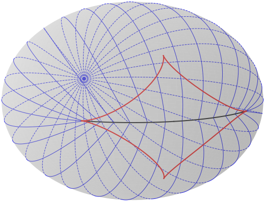
Figures
Geodesics departing from \(q_0=(0,0)\) for different \(\alpha_0 \in [0, 2\pi)\) until cut point. The conjugate locus is in red. The cut locus is represented in black. It is the segment of the equator contained in the conjugate locus. The extremities of the cut locus are cusps of the conjugate locus while interior points are isochronous separating points.
References
[Allgower-Georg 2003] E. Allgower & K. Georg, Introduction to numerical continuation methods, vol. 45 of Classics in Applied Mathematics, Soc. for Industrial and Applied Math., Philadelphia, PA, USA, (2003), 388 pages.
[Berger 2003] M. Berger, A panoramic view of Riemannian geometry, Springer, 2003.
[Bonnard et al. 2014] B. Bonnard, O. Cots & L. Jassionnesse, Geometric and numerical techniques to compute conjugate and cut loci on Riemannian surfaces, in INDAM Series vol. 5, Geometric Control and sub-Riemannian Geometry, (2014). Proceedings of the conference “Geometric Control and sub-Riemannian geometry”, Cortona, Italy, May 2012.
[Caillau et al. 2011] J.-B. Caillau, O. Cots & J. Gergaud, Differential continuation for regular optimal control problems, Optim. Methods Softw., 27 (2011), no. 2, pp. 177–196.
[do Carmo 1988] M. P. Do Carmo, Riemannian geometry, Birkhäuser, Mathematics: Theory & applications, second edn 1988.
[Facca et al. 2021] E. Facca, L. Berti, F. Fassó and M. Putti. Computing the Cut Locus of a Riemannian Manifold via Optimal Transport. 2021. ⟨hal-03467888⟩
[Hairer et al. 1993] E. Hairer, S. P. Nørsett & G. Wanner, Solving Ordinary Differential Equations I, Nonstiff Problems, vol 8 of Springer Serie in Computational Mathematics, Springer-Verlag, second edn (1993).
[Hairer-Wanner 1996] E. Hairer & G. Wanner, Solving Ordinary Differential Equations II, Stiff and Differential-Algebraic Problems, vol 14 of Springer Serie in Computational Mathematics, Springer-Verlag, second edn (1996).
[Hascoët-Pascual 2012] L. Hascoët & V. Pascual, The Tapenade Automatic Differentiation tool: principles, model, and specification, Rapport de recherche RR-7957, INRIA (2012).
[Itoh-Kiohara 2004] J. Itoh and K. Kiyohara, The cut loci and the conjugate loci on ellipsoids, Manuscripta math., 114 (2004), no. 2, pp. 247-264.
[Itoh-Sinclair 2004] J. Itoh. and R. Sinclair. Thaw: A Tool for Approximating Cut Loci on a Triangulation of a Surface. Experiment. Math. 13 (2004), no. 3, 309-325.
[Moré et al. 1980] J. J. Moré, B. S. Garbow & K. E. Hillstrom, User Guide for MINPACK-1, ANL-80-74, Argonne National Laboratory, (1980).
[Sinclair-Tanaka 2002] R. Sinclair and M. Tanaka. Loki: Software for Computing Cut Loci. Exper. Math. 11 (2002), no. 1, 1–25.
Annexes
wrappers.py
[ ]:
!pygmentize wrappers.py
plottings.py
[ ]:
!pygmentize plottings.py
bdd.py
[ ]:
!pygmentize bdd.py