Notebook source code:
examples/irrigation/irrigation.ipynb
Run the notebook yourself on binder
![]()
Optimal Control of a crop irrigation model under water Scarcity
You may find a detailed article about this problem in the following link : https://hal.archives-ouvertes.fr/hal-01991296v2
The goal of this study is to optimize the schedule of irrigation to maximize biomass production under the assumption of having a certain amount or Quota of water.
We consider the following crop irrigation model, where \(B(t)\) stands for crop biomass at time t and \(S(t)\) stands for relative sol humidity in the root zone:
with the initial conditions: \(S(0)=S_0>S_*\) and \(B(0)=B_0>0\)
The piecewise linear non decreasing from \([0,1]\) to \([0,1]\) functions \(K_R\) and \(K_S\) are defined thanks to the key constants : \(S_w\) which represents the plant wilting point, \(S_h\) which represents the hydroscopic point and \(S_*\), the minimal threshold on the soil humidity that gives the best biomass production:
\(K_S(S)\)=\(\begin{cases} 0 if S \in [0,S_w] \\ \frac{S-S_w}{S_*-S_w} if S \in [0,S_w] \\ 1 if S \in [S_*,1] \end{cases}\)
\(K_R(S)\)=\(\begin{cases} 0 if S \in [0,S_h] \\ \frac{S-S_h}{1-S_h} if S \in [S_h,1] \end{cases}\)
where 0 < \(S_h\) < \(S_w\) < \(S_*\) < 1
Therefore, our optimisation problem is:
where \(\dot V = u(t)\) and \(V(0)=0\) and the target : \(V(T)=\bar V=\frac{\bar Q}{F_{max}}\)
[6]:
using JuMP   # NLP modelling
using Ipopt  # NLP solver
using Plots  # For plotting
using PyCall # Using python libraries
[7]:
# Constants of the problem
T = 1                  # Duration of the irrigation
k_1 = 2.5
k_2 = 5
S_etoile = 0.7
S_w = 0.4
S_h = 0.2
F_max = 1.2
alpha = 3              # Using phi(t) = t^(alpha)
S_0 = 1                # Initial soil humidity
B_0 = 0                # Initial Biomass
V_0 = 0                # Initial quantity of water
t0 = 0                 # Sowing date
tf = T                 # Harvesting date
Q_bar = 0.09           # Water Quota
V_max = Q_bar/F_max    # Terminal condition on water quota

#The evaluation of the Ks function given a point S and the two thresholds S* and Sw
function KS(S)
    res = 0
    if S>=0 && S<=S_w
        res = 0
    elseif S>=S_w && S<=S_etoile
        res = (S-S_w)/(S_etoile-S_w)
    else
        res = 1
    end
    return res
end
[7]:
KS (generic function with 1 method)
Using Lagrange polynomial interpolation for smoothing the Ks function
The function \(K_S\) is nonlinear, therefore we need to smooth it in order to be able to define it in the JuMP model. This smoothing uses the Lagrange polynomial interpolation method where we choose a set of points that the polynomial should interpolate. Note that the corner points of \(K_S\) are very important in this optimization problem as you can see in the article presented above. Therefore, one should always include \(S_w\) and \(S_*\) in the set of interpolated points.
[8]:
# Calling some useful Python libraries
np = pyimport("numpy")
Interpolate = pyimport("scipy.interpolate")
Pol = pyimport("numpy.polynomial")

# Applying the Lagrange polynomial interpolation method to the function Ks in order to make it
# usable in JuMP.

# Interpolation points
# You can choose any set of points, as long as it includes the corner points Sw and S*
x = np.array([0,0.04,0.05,0.06,0.1,0.15,0.2,0.3,0.4,0.5,0.6,0.7,0.8,0.9,0.97,0.98,0.99,1,1.001])
y = np.array([KS(s) for s in x])

# The coefficients of the lagrange polynomial
# P = coef[d]*S + coef[d-1]*S² + ....... + coef[1]*S^d
poly = Interpolate.lagrange(x,y)
coef = Pol.Polynomial(poly).coef
d = size(coef, 1) - 1
println("The degree of the polynomial: $(d)\n")
println("The coefficients of the polynomial :\n ")
print(coef)
The degree of the polynomial: 18

The coefficients of the polynomial :

[-6.383217239654541e7, 5.878971698271484e8, -2.4695480669023438e9, 6.2633767616015625e9, -1.0701879900125e10, 1.301654776675e10, -1.1611603401578125e10, 7.71526900490625e9, -3.84020989959375e9, 1.4293626976445312e9, -3.9459803530249023e8, 7.964622618457031e7, -1.1510975383407593e7, 1.1573526673231125e6, -77727.29947686195, 3276.738518975675, -77.50842254672898, 0.7779864636318052, 0.0]
[9]:
# The evaluation of the Lagrange version of the function Ks on a point S
function KS_lagrange(S)
    s = 0
    n = size(coef, 1)
    for i in 1:n
        s = s + coef[i]*(S^(n-i))
    end
    return s
end

# Plotting Ks and Ks_Lagrange
N = 500
Δt = 1/N
t = (1:N) * Δt
r1 = []
r2 = []
for i in 1:N
    append!(r1, KS(t[i]))
    append!(r2, KS_lagrange(t[i]))
end

plot(t, r1, label="KS")
plot!(t, r2, label="KS_Lagrange")
[9]:

Solving the problem using the Ipopt solver
[10]:
   # JuMP model, Ipopt solver
    sys = Model(optimizer_with_attributes(Ipopt.Optimizer, "print_level" => 3))
    set_optimizer_attribute(sys, "tol", 1e-9)
    set_optimizer_attribute(sys, "max_iter", 100000)
    # Parameters

    N = 100    # grid size
    Δt = (tf-t0)/N             # Time step

    f(x, y) = max(x,y)
    JuMP.register(sys, :f, 2, f, autodiff=true)

    g(x, y) = min(x,y)
    JuMP.register(sys, :g, 2, g, autodiff=true)

    JuMP.@variables(sys, begin
        0. ≤ s[1:N] ≤ 1.       # s : soil humidty
        0. ≤ V[1:N] ≤ V_max    # V
        0. ≤ b[1:N] ≤ 1.       # B
        0. ≤ u[1:N] ≤ 1.       # allocation (control)
    end)


    # Objective
    @objective(sys, Max, b[N])

    # Initial conditions
    @constraints(sys, begin
        s[1] == S_0
        V[1] == V_0
        b[1] == B_0
        #V[N] == V_max
    end)


    # Dynamics
    @NLexpression(sys, ph[j = 1:N], (j*Δt)^alpha)
    @NLexpression(sys, Kr[j = 1:N], g(1, f(0,(s[j]-S_h)/(1-S_h))) )
    # A polynomial approxmation of Ks using Lagrange interpolation
    # P = coef[d]*S + coef[d-1]*S² + ....... + coef[1]*S^d
    @NLexpression(sys, Ks[j = 1:N], coef[d]*s[j] + coef[d-1]*(s[j]^2) + coef[d-2]*(s[j]^3) + coef[d-3]*(s[j]^4)
                                  + coef[d-4]*(s[j]^5) + coef[d-5]*(s[j]^6) + coef[d-6]*(s[j]^7) + coef[d-7]*(s[j]^8)
                                  + coef[d-8]*(s[j]^9) + coef[d-9]*(s[j]^10) + coef[d-10]*(s[j]^11) + coef[d-11]*(s[j]^12)
                                  + coef[d-12]*(s[j]^13) + coef[d-13]*(s[j]^14) + coef[d-14]*(s[j]^15) + coef[d-15]*(s[j]^16)
                                  + coef[d-16]*(s[j]^17) + coef[d-17]*(s[j]^18) )

    for j in 1:N-1
        @NLconstraint(sys, s[j+1] == s[j] +  Δt * k_1*(-ph[j]*Ks[j] - (1-ph[j])*Kr[j] + k_2*u[j]))
        @NLconstraint(sys, b[j+1] == b[j] +  Δt * ph[j]*Ks[j])
        @NLconstraint(sys, V[j+1] == V[j] +  Δt * u[j])
    end


    #Solve for the control and state
    #println("Solving...")
    status = optimize!(sys)
    #println("Solver status: ", status)
    s1 = value.(s)
    b1 = value.(b)
    V1 = value.(V)
    u1 = value.(u)
    println("Cost: ", objective_value(sys))
******************************************************************************
This program contains Ipopt, a library for large-scale nonlinear optimization.
 Ipopt is released as open source code under the Eclipse Public License (EPL).
         For more information visit https://github.com/coin-or/Ipopt
******************************************************************************

Total number of variables............................:      400
                     variables with only lower bounds:        0
                variables with lower and upper bounds:      400
                     variables with only upper bounds:        0
Total number of equality constraints.................:      300
Total number of inequality constraints...............:        0
        inequality constraints with only lower bounds:        0
   inequality constraints with lower and upper bounds:        0
        inequality constraints with only upper bounds:        0


Number of Iterations....: 81

                                   (scaled)                 (unscaled)
Objective...............:  -1.8904448217544384e-01    1.8904448217544384e-01
Dual infeasibility......:   6.1389971181453527e-09    6.1389971181453527e-09
Constraint violation....:   9.7540131527296126e-10    9.7540131527296126e-10
Complementarity.........:   5.2713078088771370e-18   -5.2713078088771370e-18
Overall NLP error.......:   6.1389971181453527e-09    6.1389971181453527e-09


Number of objective function evaluations             = 110
Number of objective gradient evaluations             = 82
Number of equality constraint evaluations            = 110
Number of inequality constraint evaluations          = 0
Number of equality constraint Jacobian evaluations   = 82
Number of inequality constraint Jacobian evaluations = 0
Number of Lagrangian Hessian evaluations             = 0
Total CPU secs in IPOPT (w/o function evaluations)   =      6.615
Total CPU secs in NLP function evaluations           =      0.494

EXIT: Solved To Acceptable Level.
Cost: 0.18904448217544384
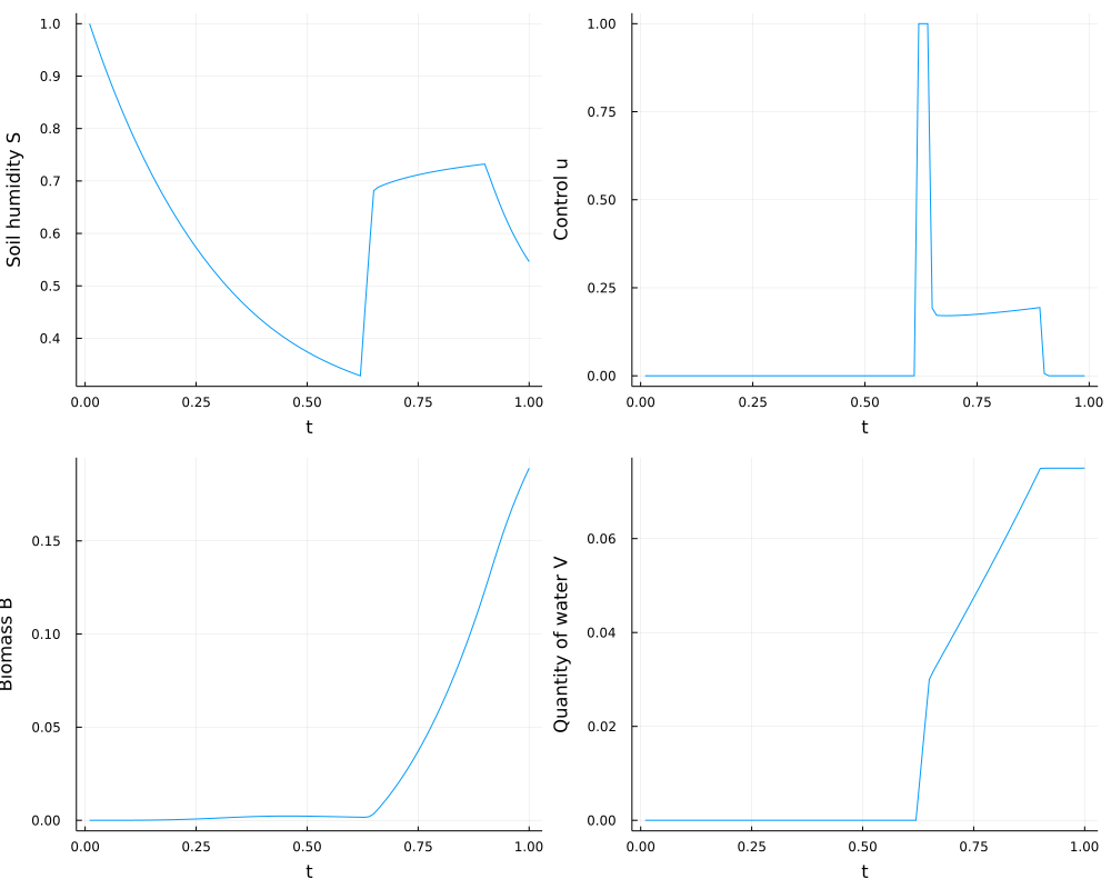
[11]:
t = (1:N) * Δt
s_plot = plot(t, s1, xlabel = "t", ylabel = "Soil humidity S", legend = false, fmt = :png)
u_plot = plot(t[1:N-1], u1[1:N-1], xlabel = "t", ylabel = "Control u", legend = false, fmt = :png)
b_plot = plot(t, b1, xlabel = "t", ylabel = "Biomass B", legend = false, fmt = :png)
v_plot = plot(t, V1, xlabel = "t", ylabel = "Quantity of water V", legend = false, fmt = :png)
display(plot(s_plot, u_plot, b_plot, v_plot, layout = (2, 2), size=(1000,800)))