Notebook source code:
examples/shooting_tutorials/multiple_shooting_homotopy.ipynb
Run the notebook yourself on binder
![]()
Homotopy and indirect multiple shooting
Author: Olivier Cots
Date: November 2021
I) Description of the optimal control problem
We consider the following optimal control problem:
To this optimal control problem is associated the stationnary optimization problem
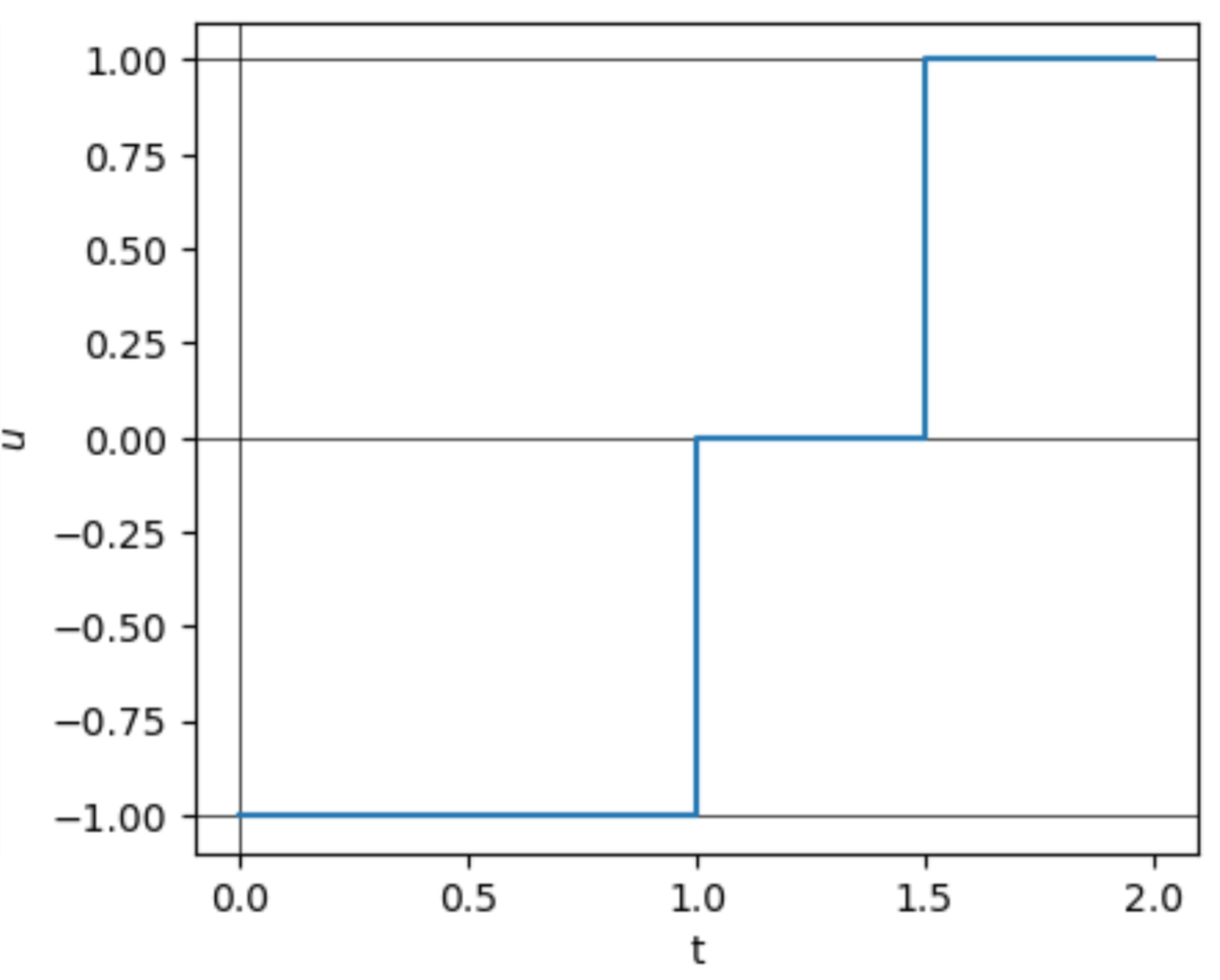
The static solution is thus \((x^*, u^*) = (0, 0)\). This solution may be seen as the static pair \((x, u)\) which minimizes the cost \(J(u)\) under the constraint \(u \in [-1, 1]\). It is well known that this problem is what we call a turnpike optimal control problem. Hence, if the final time \(t_f\) is long enough the solution is of the following form: starting from \(x(0)=1\), reach as fast as possible the static solution, stay at the static solution as long as possible before reaching the target \(x(t_f)=1/2\). In this case, the optimal control would be
with \(0 < t_1 < t_2 < t_f\). We say that the control is Bang-Singular-Bang. A Bang arc corresponds to \(u \in \{-1, 1\}\) while a singular control corresponds to \(u \in (-1, 1)\). Since the optimal control law is discontinuous, then to solve this optimal control problem by indirect methods and find the switching times \(t_1\) and \(t_2\), we need to implement what we call a multiple shooting method. In the next section we introduce a regularization technique to force the control to be in the set \((-1,1)\) and to be smooth. In this context, we will be able to implement a simple shooting method and determine the structure of the optimal control law. Thanks to the simple shooting method, we will have the structure of the optimal control law together with an approximation of the switching times that we will use as initial guess for the multiple shooting method that we present in the last section.
Main goal
Find the switching times \(t_1\) and \(t_2\) by multiple shooting.
Steps:
Regularize the problem and solve the regularized problem by simple shooting.
Determine the structure of the non-regularized optimal control problem, that is the structure Bang-Singular-Bang, and find a good approximation of the switching times and of the initial co-vector.
Solve the non-regularized optimal control problem by multiple shooting.
Remark 1. See this page for a general presentation of the simple shooting method.
Remark 2. In this particular example, the singular control does not depend on the costate \(p\) since it is constant. This happens in low dimension. This could be taken into consideration to simplify the definition of the multiple shooting method. However, to stay general, we will not consider this particular property in this notebook.
II) Regularization and simple shooting
We make the following regularization:
Our goal is to determine the structure of the optimal control problem when \((\varepsilon, t_f) = (0, 2)\). The problem is simpler to solver when \(\varepsilon\) is bigger and \(t_f\) is smaller. It is also smooth whenever \(\varepsilon>0\). Hence, we will start by solving the problem for \((\varepsilon, t_f) = (1, 1)\). In a second step, we will decrease the penalization term \(\varepsilon\) and in a final step, we will increase the final time \(t_f\) to the final value \(2\).
Preliminaries
[1]:
# import packages
import nutopy as nt
import nutopy.tools as tools
import nutopy.ocp as ocp
import numpy as np
import matplotlib.pyplot as plt
plt.rcParams['figure.figsize'] = [16, 4]
plt.rcParams['figure.dpi'] = 100
[2]:
# Finite differences function
# Return f'(x).dx
def finite_diff(fun, x, dx, *args, **kwargs):
    v_eps = np.finfo(float).eps
    t = np.sqrt(v_eps) * np.sqrt(np.maximum(1.0, np.linalg.norm(x))) / np.sqrt(np.maximum(1.0, np.linalg.norm(dx)))
    j = (fun(x + t*dx, *args, **kwargs) - fun(x, *args, **kwargs)) / t
    return j
[3]:
# Parameters

t0        = 0.0
x0        = np.array([1.0])
xf_target = np.array([0.5])

e_init    = 1.0
e_final   = 0.002 #

tf_init   = 1.0 # With this value the problem is simpler to solver since the trajectory stay
                # less time around the static solution
tf_final  = 2.0
Maximized Hamiltonian and its derivatives
The pseudo-Hamiltonian is (in the normal case)
Note that we put the parameter \(\varepsilon\) into the arguments of the pseudo-Hamiltonian since we will vary it.
[4]:
# Control in feedback form u[p,e].
#
@tools.vectorize(vvars=(1,))
def ufun(p, e):
    u = (-e + np.sqrt(e**2+p**2))/p
    return u
[5]:
# Derivative of the control in feedback form.
#
def dufun(p, dp, e, de):
    s    = np.sqrt(e**2+p**2)
    dudp = (1.0/s + (e - s)/p**2)*dp
    dude = finite_diff(lambda e_: ufun(p, e_), e, de)
    du   = dudp+dude
    return du

ufun = tools.tensorize(dufun, tvars=(1,2))(ufun)
We give next the maximized Hamiltonian with its derivatives. This permits us to define the flow of the associated Hamiltonian vector field.
[6]:
# Definition of the maximized Hamiltonian and its derivatives
# The second derivative d2hfun is computed by finite differences for a part
def dhfun(t, x, dx, p, dp, e, de):
    # dh = dh_x dx + dh_p dp
    u, du  = ufun((p, dp), (e, de))
    hd     = dp*u + p*du - 2*x*dx + de*(np.log(1.0-u**2)) - e*(2.0*u*du)/(1.0-u**2)
    return hd

def d2hfun(t, x, dx, d2x, p, dp, d2p, e, de, d2e):
    d2h_xx = -2.0*dx*d2x # d2h_dxx dx d2x
    #
    phi_p  = lambda p_: dhfun(t, x, 0.0, p_, dp, e, de) # dh_dx does not depend on p so dx=0
    phi_e  = lambda e_: dhfun(t, x, 0.0, p, dp, e_, de) # dh_dx does not depend on p so dx=0
    #
    dphi_p = finite_diff(phi_p, p, d2p)
    dphi_e = finite_diff(phi_e, e, d2e)
    #
    hdd    = d2h_xx + dphi_p + dphi_e
    return hdd

@tools.tensorize(dhfun, d2hfun, tvars=(2, 3, 4))
def hfun(t, x, p, e):
    u = ufun(p, e)
    h = p*u - x**2 + e*(np.log(1.0-u**2))
    return h

h = ocp.Hamiltonian(hfun)   # The Hamiltonian object

f = ocp.Flow(h)             # The flow associated to the Hamiltonian object is
                            # the exponential mapping with its derivative
                            # that can be used to define the Jacobian of the
                            # shooting function
Shooting function and its derivative
The shooting function is
where \(z(t_f, x_0, p_0, \varepsilon)\) is the solution of the associated Hamiltonian system with the initial condition \(z(0) = (x_0, p_0)\). Note that the Hamiltonian system depends on \(\varepsilon\). We put \(\varepsilon\) and \(t_f\) into the arguments of the shooting function since we will vary them.
Procedure
First solve \(S=0\) for \((\varepsilon, t_f) = (1,1)\) then decrease \(\varepsilon\) to \(0.002\), and finish by increasing \(t_f\) to 2.
[7]:
# Definition of the shooting function
#
def shoot(p0, e, tf):
    xf, _ = f(t0, x0, p0, tf, e)  # We use the flow to get z(tf, x0, p0)
    s = xf - xf_target  # x(tf, x0, p0) - xf_target
    return s
[8]:
# Derivative of the shooting function
#
def dshoot(p0, dp0, e, tf):
    (xf, dxf), _ = f(t0, x0, (p0, dp0), tf, e)
    ds = dxf
    return ds

shoot = nt.tools.tensorize(dshoot, tvars=(1,))(shoot)
[9]:
# Function to plot the solution
def plotSolution(p0, e, tf):

    N      = 200
    tspan  = list(np.linspace(t0, tf, N+1))
    xf, pf = f(t0, x0, p0, tspan, e)
    u      = ufun(pf, e)

    fig = plt.figure()
    ax  = fig.add_subplot(131); ax.plot(tspan, xf); ax.set_xlabel('t'); ax.set_ylabel('$x$'); ax.axhline( 0, color='k', linewidth=0.5); ax.axvline( 0, color='k', linewidth=0.5)
    ax  = fig.add_subplot(132); ax.plot(tspan, pf); ax.set_xlabel('t'); ax.set_ylabel('$p$'); ax.axhline( 0, color='k', linewidth=0.5); ax.axvline( 0, color='k', linewidth=0.5)
    ax  = fig.add_subplot(133); ax.plot(tspan,  u); ax.set_xlabel('t'); ax.set_ylabel('$u$'); ax.axhline( 0, color='k', linewidth=0.5); ax.axvline( 0, color='k', linewidth=0.5)

    ax.axhline(-1, color='k', linewidth=0.5)
    ax.axhline( 1, color='k', linewidth=0.5)
Resolution of the regularized problem
[10]:
# Shooting for (tf, e) = (tf_init, e_init)
p0_guess = np.array([0.1])
nlefun   = lambda p0: shoot(p0, e_init, tf_init)
sol_nle  = nt.nle.solve(nlefun, p0_guess, df=nlefun)
     Calls  |f(x)|                 |x|

         1  9.225527956247914e-01  1.000000000000000e-01
         2  1.328510077221831e-01  2.933843266521996e+00
         3  7.295873938738073e-02  2.551952341029376e+00
         4  3.048709516367498e-02  2.086745707818067e+00
         5  4.420525603090641e-03  2.223849332715463e+00
         6  2.283581438740634e-04  2.206487218918453e+00
         7  1.831091399617790e-06  2.205541459924093e+00
         8  7.509122768034615e-10  2.205548983174078e+00
         9  2.775557561562891e-15  2.205548980090132e+00

 Results of the nle solver method:

 xsol    =  [-2.20554898]
 f(xsol) =  [-2.77555756e-15]
 nfev    =  9
 njev    =  1
 status  =  1
 success =  True

 Successfully completed: relative error between two consecutive iterates is at most TolX.
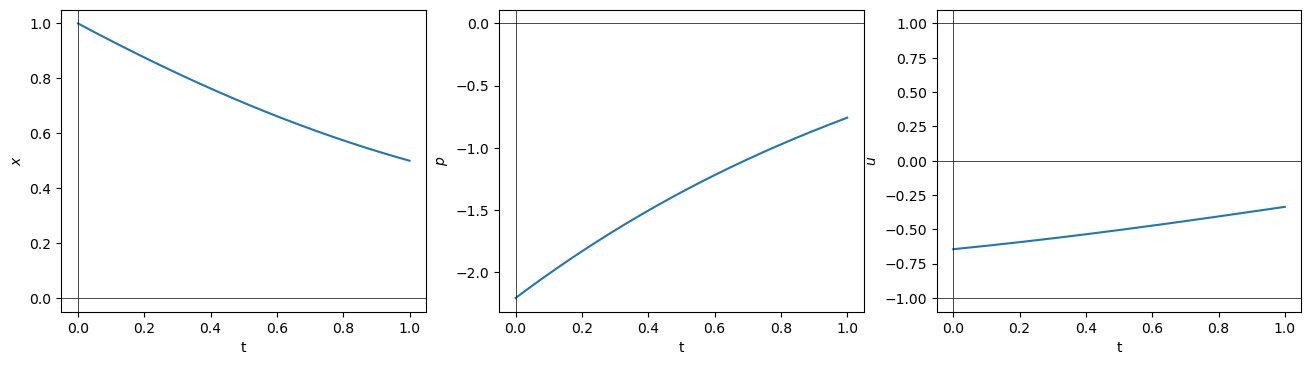
[11]:
# Plot solution for (tf, e) = (tf_init, e_init)
plotSolution(sol_nle.x, e_init, tf_init)
[12]:
# Definition of the homotopic function and its first order derivative
# This function is used to solve S=0 for different values of e=epsilon and tf.
def dhomfun(p0, dp0, e, de, tf, dtf):
    (xf, dxf), (pf, dpf) = f(t0, x0, (p0, dp0), (tf, dtf), (e, de))
    s  = xf - xf_target
    ds = dxf
    return s, ds

@tools.tensorize(dhomfun, tvars=(1, 2, 3), full=True)
def homfun(p0, e, tf):
    xf, pf = f(t0, x0, p0, tf, e)  # We use the flow to get z(tf, x0, p0, e)
    s = xf - xf_target             # x(tf, x0, p0) - xf_target
    return s
[13]:
# Making the penalization smaller: homotopy on e
p0         = sol_nle.x
sol_path_e = nt.path.solve(homfun, p0, e_init, e_final, args=tf_init, df=homfun)
     Calls  |f(x,pars)|     |x|                Homotopic param    Arclength s     det A(s)        Dot product

         1  2.22044605e-16  2.20554898009e+00  1.00000000000e+00  0.00000000e+00 -3.99453535e-01  0.00000000e+00
         2  1.11022302e-16  2.19703976143e+00  9.93456169344e-01  1.07344549e-02 -4.02221682e-01  9.99999991e-01
         3  1.11022302e-16  2.17091059635e+00  9.73350710885e-01  4.37035729e-02 -4.10968794e-01  9.99999912e-01
         4  0.00000000e+00  2.10847891252e+00  9.25237575324e-01  1.22523555e-01 -4.33507698e-01  9.99999404e-01
         5  1.11022302e-16  1.99082951629e+00  8.34243096651e-01  2.71256157e-01 -4.83546064e-01  9.99996934e-01
         6  3.33066907e-16  1.86334364794e+00  7.35036720733e-01  4.32794321e-01 -5.52818042e-01  9.99993861e-01
         7  1.66533454e-16  1.73133423638e+00  6.31424683702e-01  6.00609682e-01 -6.49305052e-01  9.99987907e-01
         8  1.66533454e-16  1.61006281732e+00  5.35152931092e-01  7.55448578e-01 -7.73371470e-01  9.99980850e-01
         9  1.11022302e-16  1.51382082812e+00  4.57748930613e-01  8.78955472e-01 -9.11191192e-01  9.99979147e-01
        10  7.77156117e-16  1.41954327767e+00  3.80805609795e-01  1.00064609e+00 -1.10190408e+00  9.99969075e-01
        11  3.88578059e-16  1.33395167905e+00  3.09795044097e-01  1.11185980e+00 -1.35386473e+00  9.99967740e-01
        12  8.88178420e-16  1.27252535918e+00  2.58131862126e-01  1.19212369e+00 -1.60870726e+00  9.99986804e-01
        13  1.11022302e-16  1.22355088827e+00  2.16626266915e-01  1.25632038e+00 -1.87815450e+00  9.99997628e-01
        14  1.11022302e-16  1.18286379372e+00  1.82100667179e-01  1.30968195e+00 -2.16402578e+00  9.99999424e-01
        15  1.11022302e-16  1.14808642199e+00  1.52752248613e-01  1.35518798e+00 -2.46801360e+00  9.99990065e-01
        16  1.22124533e-15  1.11795888116e+00  1.27640006041e-01  1.39440916e+00 -2.78989695e+00  9.99969980e-01
        17  2.22044605e-16  1.09169067747e+00  1.06152515592e-01  1.42834648e+00 -3.12889830e+00  9.99942600e-01
        18  5.55111512e-17  1.06868078573e+00  8.77861370232e-02  1.45778781e+00 -3.48484627e+00  9.99912527e-01
        19  7.77156117e-16  1.04847323663e+00  7.21227238411e-02  1.48335537e+00 -3.85774779e+00  9.99883959e-01
        20  7.77156117e-16  1.03068325887e+00  5.87839947123e-02  1.50559085e+00 -4.24823183e+00  9.99859387e-01
        21  2.22044605e-16  1.01502219607e+00  4.74602185802e-02  1.52491717e+00 -4.65642725e+00  9.99840540e-01
        22  1.11022302e-15  1.00123717495e+00  3.78707784108e-02  1.54170980e+00 -5.08270248e+00  9.99827498e-01
        23  1.88737914e-15  9.89141096616e-01  2.97889404625e-02  1.55625756e+00 -5.52631818e+00  9.99820609e-01
        24  6.10622664e-16  9.78564899170e-01  2.30096164772e-02  1.56882020e+00 -5.98633192e+00  9.99818989e-01
        25  2.33146835e-15  9.69381178860e-01  1.73654413577e-02  1.57959985e+00 -6.46020938e+00  9.99822504e-01
        26  2.44249065e-15  9.61478540542e-01  1.27092564228e-02  1.58877232e+00 -6.94420988e+00  9.99830409e-01
        27  1.13797860e-14  9.54783151738e-01  8.92568307915e-03  1.59646291e+00 -7.43119477e+00  9.99843159e-01
        28  1.21014310e-14  9.49229594793e-01  5.91232630285e-03  1.60278140e+00 -7.91109577e+00  9.99860325e-01
        29  8.88178420e-16  9.44800393396e-01  3.59993850183e-03  1.60777794e+00 -8.36564427e+00  9.99883773e-01
        30  2.40918396e-14  9.41628939496e-01  2.00000000000e-03  1.61133012e+00 -8.74974014e+00  9.99921341e-01

 Results of the path solver method:

 xf            =  [-0.94162894]
 parsf         =  0.002
 |f(xf,parsf)| =  2.4091839634365897e-14
 steps         =  30
 status        =  1
 success       =  True

 Homotopy successfully completed.
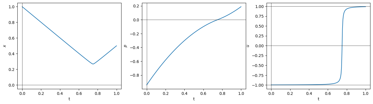
[14]:
# Plot solution for (tf, e) = (tf_init, e_final)
plotSolution(sol_path_e.xf, e_final, tf_init)
[15]:
# Making the time bigger: homotopy on tf
p0          = sol_path_e.xf                       # sol is coming from last homotopy
pathfun     = lambda p0, tf, e: homfun(p0, e, tf) # invert order of arguments
sol_path_tf = nt.path.solve(pathfun, p0, tf_init, tf_final, args=e_final, df=pathfun)
     Calls  |f(x,pars)|     |x|                Homotopic param    Arclength s     det A(s)        Dot product

         1  3.33066907e-16  9.41628939496e-01  1.00000000000e+00  0.00000000e+00  4.01455616e+00  0.00000000e+00
         2  6.66133815e-16  9.44075168783e-01  1.00970881515e+00  1.00122571e-02  4.08611499e+00  9.99990246e-01
         3  1.99840144e-15  9.52568966522e-01  1.04493836947e+00  4.62516611e-02  4.37006199e+00  9.99870687e-01
         4  7.77156117e-15  9.62039208912e-01  1.08753264670e+00  8.98867215e-02  4.77386771e+00  9.99809223e-01
         5  5.55111512e-16  9.72422987607e-01  1.13954563511e+00  1.42927348e-01  5.38493337e+00  9.99713845e-01
         6  2.22044605e-15  9.81702197846e-01  1.19268928589e+00  1.96876361e-01  6.19714547e+00  9.99701774e-01
         7  1.11022302e-15  9.89591429236e-01  1.24538499788e+00  2.50160646e-01  7.28195337e+00  9.99710682e-01
         8  1.99840144e-15  9.95884976491e-01  1.29533898297e+00  3.00510582e-01  8.70987139e+00  9.99747427e-01
         9  3.44169138e-15  1.00074706996e+00  1.34199933084e+00  3.47424387e-01  1.06098834e+01  9.99790135e-01
        10  7.77156117e-16  1.00439208643e+00  1.38505432086e+00  3.90633992e-01  1.31673457e+01  9.99834099e-01
        11  5.44009282e-15  1.00706227821e+00  1.42461082683e+00  4.30280935e-01  1.66709868e+01  9.99874139e-01
        12  2.77555756e-16  1.00897681973e+00  1.46091117805e+00  4.66632016e-01  2.15645706e+01  9.99908583e-01
        13  2.44249065e-15  1.01032317760e+00  1.49430901164e+00  5.00057153e-01  2.85458054e+01  9.99936600e-01
        14  1.98729921e-14  1.01125311245e+00  1.52521134131e+00  5.30973579e-01  3.87278283e+01  9.99958208e-01
        15  3.85247390e-14  1.01188503157e+00  1.55405907535e+00  5.59828296e-01  5.39233219e+01  9.99973924e-01
        16  1.08357767e-13  1.01230818019e+00  1.58130984382e+00  5.87082385e-01  7.71529196e+01  9.99984648e-01
        17  1.79301018e-13  1.01258776709e+00  1.60742756300e+00  6.13201619e-01  1.13588859e+02  9.99991489e-01
        18  3.01203507e-13  1.01277014591e+00  1.63287675550e+00  6.38651474e-01  1.72371687e+02  9.99995562e-01
        19  3.67372799e-13  1.01288752233e+00  1.65812118466e+00  6.63896181e-01  2.70247999e+02  9.99997826e-01
        20  3.82471832e-13  1.01296189377e+00  1.68362881730e+00  6.89403924e-01  4.39194297e+02  9.99999002e-01
        21  5.13478149e-14  1.01300810960e+00  1.70988219910e+00  7.15657347e-01  7.43230516e+02  9.99999573e-01
        22  4.68775019e-12  1.01303611851e+00  1.73739507141e+00  7.43170234e-01  1.31775647e+03  9.99999831e-01
        23  2.76326739e-11  1.01305254843e+00  1.76673610983e+00  7.72511278e-01  2.46810170e+03  9.99999938e-01
        24  1.36599621e-10  1.01306178557e+00  1.79856204066e+00  8.04337210e-01  4.93701447e+03  9.99999980e-01
        25  7.16485427e-10  1.01306670035e+00  1.83366524984e+00  8.39440419e-01  1.07030407e+04  9.99999994e-01
        26  4.28382685e-09  1.01306913478e+00  1.87304471211e+00  8.78819882e-01  2.56514463e+04  9.99999999e-01
        27  3.21707785e-08  1.01307023317e+00  1.91801646616e+00  9.23791636e-01  6.98430599e+04  1.00000000e+00
        28  3.30288299e-07  1.01307067137e+00  1.97039116143e+00  9.76166331e-01  2.24369157e+05  1.00000000e+00
        29  2.38883633e-06  1.01307076680e+00  2.00000000000e+00  1.00577516e+00  4.36366061e+05  1.00000000e+00

 Results of the path solver method:

 xf            =  [-1.01307077]
 parsf         =  2.0
 |f(xf,parsf)| =  2.3888363341884045e-06
 steps         =  29
 status        =  1
 success       =  True

 Homotopy successfully completed.
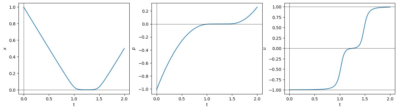
[16]:
# Plot solution for (tf, e) = (tf_final, e_final)
plotSolution(sol_path_tf.xf, e_final, tf_final)
III) Resolution of the optimal control problem by multiple shooting
We come back to the original optimal control problem:
We have determined that the optimal control follows the strategy:
with \(0 < t_1 < t_2 < t_f=2\).
Goal
The goal is to find the values of the switching times \(t_1\) and \(t_2\) together with the initial covector \(p_0\) (see Remark 2).
Maximized Hamiltonian and its derivatives
We define first the three control laws \(u \equiv \{-1, 0, 1\}\).
[17]:
# Controls in feedback form
@tools.vectorize(vvars=(1, 2, 3))
def uplus(t, x, p):
    u = +1.0
    return u

@tools.vectorize(vvars=(1, 2, 3))
def uminus(t, x, p):
    u = -1.0
    return u

@tools.vectorize(vvars=(1, 2, 3))
def using(t, x, p):
    u = 0.0
    return u
The pseudo-Hamiltonian is
[18]:
# Definition of the Hamiltonian and its derivatives for u = 1
#
def dhfunplus(t, x, dx, p, dp):
    # dh = dh_x dx + dh_p dp
    u  = uplus(t, x, p)
    hd = u*dp - 2.0*x*dx
    return hd

def d2hfunplus(t, x, dx, d2x, p, dp, d2p):
    # d2h = dh_xx dx d2x + dh_xp dp d2x + dh_px dx d2p + dh_pp dp d2p
    hdd    = -2.0 * d2x * dx
    return hdd

@tools.tensorize(dhfunplus, d2hfunplus, tvars=(2, 3))
def hfunplus(t, x, p):
    u = uplus(t, x, p)
    h = p*u - x**2
    return h

hplus = ocp.Hamiltonian(hfunplus)
fplus = ocp.Flow(hplus)
We give the Hamiltonians for \(u=-1\) and \(u=0\) with their derivatives.
[19]:
# Definition of the Hamiltonian and its derivatives for u = -1
def dhfunminus(t, x, dx, p, dp):
    # dh = dh_x dx + dh_p dp
    u  = uminus(t, x, p)
    hd = u*dp - 2.0*x*dx
    return hd

def d2hfunminus(t, x, dx, d2x, p, dp, d2p):
    # d2h = dh_xx dx d2x + dh_xp dp d2x + dh_px dx d2p + dh_pp dp d2p
    hdd    = -2.0 * d2x * dx
    return hdd

@tools.tensorize(dhfunminus, d2hfunminus, tvars=(2, 3))
def hfunminus(t, x, p):
    u = uminus(t, x, p)
    h = p*u - x**2
    return h

hminus = ocp.Hamiltonian(hfunminus)
fminus = ocp.Flow(hminus)
[20]:
# Definition of the Hamiltonian and its derivatives for u = 0
def dhfunsing(t, x, dx, p, dp):
    # dh = dh_x dx + dh_p dp
    u  = using(t, x, p)
    hd = u*dp - 2.0*x*dx
    return hd

def d2hfunsing(t, x, dx, d2x, p, dp, d2p):
    # d2h = dh_xx dx d2x + dh_xp dp d2x + dh_px dx d2p + dh_pp dp d2p
    hdd    = -2.0 * d2x * dx
    return hdd

@tools.tensorize(dhfunsing, d2hfunsing, tvars=(2, 3))
def hfunsing(t, x, p):
    u = using(t, x, p)
    h = p*u - x**2
    return h

hsing = ocp.Hamiltonian(hfunsing)
fsing = ocp.Flow(hsing)
Shooting function
The multiple shooting function is given by
where \(z_2 := (x_2, p_2) = z(t_2, t_1, x_1, p_1, u_0)\), \(z_1 := (x_1, p_1) = z(t_1, t_0, x_0, p_0, u_-)\) and where z(t, s, a, b, u) is the solution at time \(t\) of the Hamiltonian system associated to the control u starting at time \(s\) at the initial condition \(z(s) = (a,b)\).
We have introduced the notation \(u_-\) for \(u\equiv -1\), \(u_0\) for \(u\equiv 0\) and \(u_+\) for \(u\equiv +1\).
Remark: We know that \((x_2, p_2)=(0,0)\).
[21]:
# Multiple shooting function
#

tf = tf_final # we set the final time to the value tf_final

def shoot_multiple(y):
    p0 = y[0]
    t1 = y[1]
    t2 = y[2]

    x1, p1 = fminus(t0, x0, p0, t1)  # on [ 0, t1]
    x2, p2 =  (np.array([0.0]), np.array([0.0])) # or fsing(t1, x1, p1, t2)  # on [t1, t2]
    xf, pf =  fplus(t2, x2, p2, tf)  # on [t2, tf]

    s = np.zeros([3])
    s[0] = x1
    s[1] = p1
    s[2] = xf - xf_target  # x(tf, x0, p0) - xf_target
    return s
Resolution of the shooting function
[22]:
# Initial guess for the Newton solver

t1_guess = 0.9
t2_guess = 1.6

p0_guess = sol_path_tf.xf # from previous homotopy
[23]:
# Resolution of the shooting function
y_guess  = np.array([float(p0_guess), t1_guess, t2_guess])
sol_nle_mul  = nt.nle.solve(shoot_multiple, y_guess)
     Calls  |f(x)|                 |x|

         1  1.432908241330901e-01  2.096738509815840e+00
         2  9.999997231646155e-03  2.066422027534561e+00
         3  1.506879908777304e-05  2.061545503373235e+00
         4  1.103237380050136e-11  2.061552812814182e+00
         5  2.548110389416817e-16  2.061552812808831e+00

 Results of the nle solver method:

 xsol    =  [-1.   1.   1.5]
 f(xsol) =  [-2.08166817e-16 -9.62771529e-17  1.11022302e-16]
 nfev    =  5
 njev    =  1
 status  =  1
 success =  True

 Successfully completed: relative error between two consecutive iterates is at most TolX.
[24]:
# function to plot solution

def plotSolutionBSB(p0, t1, t2, tf):

    N      = 20

    tspan1  = list(np.linspace(t0, t1, N+1))
    tspan2  = list(np.linspace(t1, t2, N+1))
    tspanf  = list(np.linspace(t2, tf, N+1))

    x1, p1 = fminus(t0, x0, p0, tspan1)  # on [ 0, t1]
    x2, p2 =  fsing(t1, x1[-1], p1[-1], tspan2)  # on [t1, t2]
    xf, pf =  fplus(t2, x2[-1], p2[-1], tspanf)  # on [t2, tf]

    u1     = uminus(tspan1, x1, p1)
    u2     =  using(tspan2, x2, p2)
    uf     =  uplus(tspanf, xf, pf)

    fig = plt.figure()

    ax  = fig.add_subplot(131);
    ax.plot(np.concatenate((tspan1, tspan2, tspanf)), np.concatenate((x1, x2, xf)))
    ax.set_xlabel('t'); ax.set_ylabel('$x$'); ax.axhline(0, color='k', linewidth=0.5); ax.axvline( 0, color='k', linewidth=0.5)

    ax  = fig.add_subplot(132);
    ax.plot(np.concatenate((tspan1, tspan2, tspanf)), np.concatenate((p1, p2, pf)))
    ax.set_xlabel('t'); ax.set_ylabel('$p$'); ax.axhline(0, color='k', linewidth=0.5); ax.axvline( 0, color='k', linewidth=0.5)

    ax  = fig.add_subplot(133);
    ax.set_xlabel('t'); ax.set_ylabel('$u$'); ax.axhline(0, color='k', linewidth=0.5); ax.axvline( 0, color='k', linewidth=0.5)
    ax.axhline(-1, color='k', linewidth=0.5)
    ax.axhline( 1, color='k', linewidth=0.5)
    ax.plot(np.concatenate((tspan1, tspan2, tspanf)), np.concatenate((u1, u2, uf)))
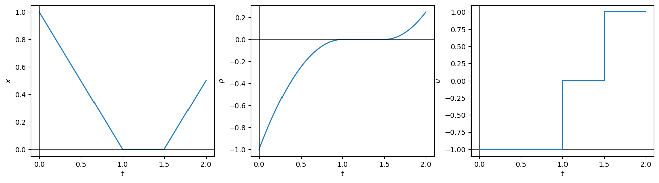
[25]:
# plot solution
p0 = sol_nle_mul.x[0]
t1 = sol_nle_mul.x[1]
t2 = sol_nle_mul.x[2]
plotSolutionBSB(p0, t1, t2, tf)
[ ]: