Notebook source code:
examples/sir/SIR.ipynb
Run the notebook yourself on binder
![]()
SIR model
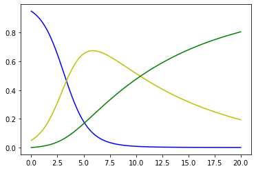
We consider a simple SIR compartmental model to describe the evolution of an infectious disease. The SIR model consists of three compartments: S for the proportion of susceptible individuals in a given population, I for the proportion of infectious and R for the proportion of recovered. We denote by p the rate of infection, which depends on the contagiousness of the virus and the density of the population (that is the contacts between individuals), and by \(\alpha\) the rate of recovery per unit of time. Then, the dynamics is
\[\begin{split}\begin{align}
\dot{S} & = -pIS \\
\dot{I} & = pIS - \alpha I \\
\dot{R} & = \alpha I
\end{align}\end{split}\]
[1]:
import numpy as np
import matplotlib.pyplot as plt
from nutopy import ivp
[2]:
def sir(t, x, pars):
    S, I, R = x
    p, alpha = pars
    y = np.zeros(x.size)
    y[0] = -p*I*S
    y[1] =  p*I*S - alpha*I
    y[2] = alpha*I
    return y
[3]:
S0 = 0.95 # initial proportion of susceptible individuals
I0 = 0.05 # initial proportion of infectious individuals
R0 = 0.00 # initial proportion of recovered individuals
x0 = np.array([S0, I0, R0])

t0 = 0.0  # initial time
tf = 20.0 # final time

p     = 1.0 # rate of infection, depending on the contagiousness
            # of the virus and the density of the population
alpha = 0.1 # rate of recovery per unit of time
pars  = np.array([p, alpha])
[4]:
sol = ivp.exp(sir, tf, t0, x0, pars)

time = sol.tout

S = sol.xout[:,0]
I = sol.xout[:,1]
R = sol.xout[:,2]
[5]:
plt.plot(time, S, 'b', time, I, 'y', time, R, 'g');