Notebook source code:
examples/smooth_case/smooth_case.ipynb
Run the notebook yourself on binder
![]()
Smooth case (direct method + shooting)
Consider the following optimal control problem (Lagrange cost, fixed final time):
with \(q\) and \(v\) fixed at \(t=0\) and \(t=1\):
Denoting \(x=(q, v)\), the Lagrange cost functional is defined by
while the dynamics is
Denoting \(p=(p_q,p_v)\), in the normal case (\(p^0=-1/2\)), the dynamic feedback is \(u=p_v\), so the maximized Hamiltonian of the problem is
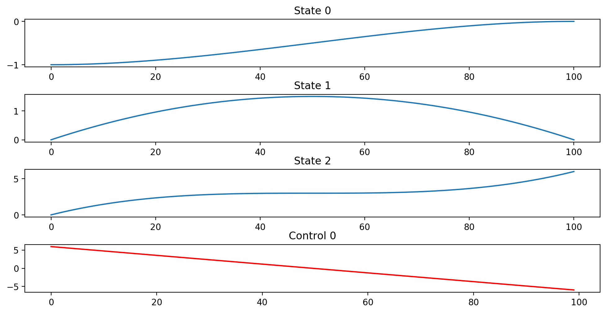
First solve: BOCOP
The problem is first solved by a so-called ‘direct transcription’ approach that discretizes the original OCP as an NLP problem. Then we use the Lagrange multipliers of this problem as a starting guess for the initial value of the costate for shooting.
[2]:
import numpy as np
import matplotlib.pyplot as plt
plt.rcParams['figure.figsize'] = [10, 5]
plt.rcParams['figure.dpi'] = 200
import os
import bocop
bocop_root_path = os.path.dirname(bocop.__file__)
print(bocop_root_path)

problem_path = bocop_root_path+"/examples/smooth_case"
print(problem_path)
solution = bocop.solve(problem_path, clean=1, debug=0, graph=2, verbose=1, cmake_options = '-DCMAKE_CXX_COMPILER=g++')

print("Bocop returns status {} with objective {:2.4g} and constraint violation {:2.4g}".format(solution.status,solution.objective,solution.constraints))
p0 = np.zeros(solution.dim_state-1) # the costate associated with the cost is not included
p0[:] = solution.costate[:-1, 0]
print("Costate at first time stage (t0+h/2): ",p0)
print("Multipliers for initial conditions: ",solution.boundarycond_multipliers[0:solution.dim_state-1])
Done
Loading solution:  /home/martinon/bocop/bocop3/bocop/examples/smooth_case/problem.sol
Bocop returns status 0 with objective 6.001 and constraint violation 1.15e-14
Costate at first time stage (t0+h/2):  [12.00120012  5.88058806]
Multipliers for initial conditions:  [12.00120012  6.00060006]
Second solve: shooting
To encode and solve the problem we use standard libraries such as numpy and pyplot, plus nutopy:
nutopy.nleis a Nonlinear Equation solvernutopy.toolsincludes@tensorizeand@vectorizedecorators (see further)nutopy.ocpdefines some useful classes and methods to manipulate optimal control problems and related stuff (Hamiltonians, flows…)
The initialization for the shooting method, an initial value for the unknown adjoint state \(p_0\), is taken from BOCOP.
[2]:
import time
from nutopy import nle
from nutopy import tools
from nutopy import ocp

t0 = 0.
x0 = np.array([ -1., 0. ])
lbda = 0.
tf = 1.
xf_fixed = np.array([ 0., 0. ]) # target is xf = (0, 0)
Hamiltonian
The (normal and maximized) Hamiltonian is straightforwardly implemented, see hfun. The code requires that its first and second derivatives wrt. to state (\(x\)) and costate (\(p\)) are also provided. This derivatives, evaluated against first and second order increments are implemented by dhfun and d2hfun, respectively. These codes can be obtained through automatic differentiation for more complicated examples (see
here, e.g.)
[3]:
def dhfun(t, x, dx, p, dp, lbda):
    q, v = x
    pq, pv = p
    qd, vd = dx
    pqd, pvd = dp
    hd = 2*pv*pvd/2. + v*pqd + pq*vd - lbda*(v**2*pvd+pv*2*v*vd)
    return hd

def d2hfun(t, x, dx, d2x, p, dp, d2p, lbda):
    q, v = x
    pq, pv = p
    qd, vd = dx
    pqd, pvd = dp
    qd0, vd0 = d2x
    pqd0, pvd0 = d2p
    hdd = pvd*2*pvd0/2. + pqd*vd0 + vd*pqd0 - lbda*(pvd*2*v*vd0+vd*2*(v*pvd0+pv*vd0))
    return hdd

@tools.tensorize(dhfun, d2hfun, tvars=(2, 3))
def hfun(t, x, p, lbda):
    q, v = x
    pq, pv = p
    h = pv**2/2. + pq*v - lbda*pv*v**2
    return h

h1 = ocp.Hamiltonian(hfun)
Note the use of the decorator @tensorize when defining hfun, after having defined its first and second derivatives. Passing the two positional arguments (dhfun, d2hfun) entails that hfun derivatives are provided up to order two, wrt. to variables specified by the named argument tvars: derivatives wrt. \(x\) and \(p\) (argument no. 2 and 3 of hfun, respectively). The decorated hfun function now contains its first and second derivative:
to evaluate \(H\) at \((t_0,x_0,p_0,\lambda)\), type
hfun(t0, x0, p0, lbda)
to evaluate \(\partial_x H\) at the same point evaluated against vector \(\mathrm{d}x_0=(2.1,-3.2)\), type
hfun(t0, (x0, dx0), p0, lbda)
to evaluate \(\partial^2_{px} H\) at the same point evaluated against vectors \(\mathrm{d}x_0=(2.1,-3.2)\) and \(\mathrm{d}p_0=(3.1,-7)\), type
hfun(t0, (x0, dx0, np.zeros(2)), (p0, np.zeros(2), dp0), lbda)
and so on for further derivatives.
Having defined the object h1 of class Hamiltonian allows to evaluate \(H\) as before, its symplectic gradient \(\vec{H}\) (h1.vec), and more.
[4]:
dx0 = np.array([ 2.1, -3.2 ])
dp0 = np.array([ 3.1, -7 ])
print( h1(t0, x0, p0, lbda) )
print( h1(t0, (x0, dx0), p0, lbda) )
print( h1(t0, (x0, dx0, np.zeros(2)), (p0, np.zeros(2), dp0), lbda) )
# and also...
print( h1.vec(t0, x0, p0, lbda) )
17.290657958685152
(17.290657958685152, -38.4038403840384)
(17.290657958685152, -38.4038403840384, -9.920000000000002)
[  0.           5.88058806   0.         -12.00120012]
An alternative way of defining the maximized Hamiltonian is to set up an optimal control problem, that is an object of type OCP, and then to use the class method fromOCP. To set an OCP, the user needs to provide the function \(f^0\) (Lagrange cost) and the dynamics \(f\). These two functions are given below, as well as their
derivatives up to order two. (Note the same use of @tensorize as before.) The user must also provide the dynamic feedback that expresses \(u\) as a function of \(x\) and \(p\), as a result of Hamiltonian maximization wrt. \(u\). Here,
In more complicated examples, there are several maximisers (including, e.g., bang and singular controls) and so several competing Hamiltonians to define using the same process. The expression h2 = Hamiltonian.fromOCP(o, ufun, -0.5) returns the (tensorized to order two) computation
with \(p^0=-1/2\) (normal case). The resulting Hamiltonian object h2 can be used exactly as the previously defined h1.
[5]:
def df0fun(t, x, dx, u, du, lbda):
    df0 = 2.*u*du
    return df0

def d2f0fun(t, x, dx, d2x, u, du, d2u, lbda):
    d2f0 = 2.*d2u*du
    return d2f0

@tools.tensorize(df0fun, d2f0fun, tvars=(2, 3))
def f0fun(t, x, u, lbda):
    f0 = u**2
    return f0

def dffun(t, x, dx, u, du, lbda):
    q, v = x
    dq, dv = dx
    df = np.zeros(2)
    df[0] = dv
    df[1] = -lbda*2.*v*dv + du
    return df

def d2ffun(t, x, dx, d2x, u, du, d2u, lbda):
    q, v = x
    dq, dv = dx
    d2q, d2v = d2x
    d2f = np.zeros(2)
    d2f[0] = 0
    d2f[1] = -lbda*2.*d2v*dv
    return d2f

@tools.tensorize(dffun, d2ffun, tvars=(2, 3))
def ffun(t, x, u, lbda):
    q, v = x
    f = np.zeros(2)
    f[0] = v
    f[1] = -lbda*v**2 + u
    return f

o = ocp.OCP(f0fun, ffun)

def dufun(t, x, dx, p, dp, lbda):
    dpq, dpv = dp
    du = dpv
    return du

def d2ufun(t, x, dx, d2x, p, dp, d2p, lbda):
    d2pq, d2pv = d2p
    d2u = 0.
    return d2u

@tools.tensorize(dufun, d2ufun, tvars=(2, 3))
def ufun(t, x, p, lbda):
    pq, pv = p
    u = pv
    return u

h2 = ocp.Hamiltonian.fromOCP(o, ufun, -0.5)
Shooting function
To define the shooting function, one must integrate the Hamiltonian system defined by h1 (or equivalently h2). This is done by defining a Flow object:
[6]:
f = ocp.Flow(h2) # h1 or h2
To compute the value of the Hamiltonan flow at time \(t_f\) starting from time \(t_0\) and initial conditions \((x_0,p_0)\) (and parameter \(\lambda\)), do the following:
[7]:
xf, pf = f(t0, x0, p0, tf, lbda)
print(xf, pf)
[-0.05990599 -0.120012 ] [12.00120012 -6.12061206]
Of course, Flow is tensorized, so you can compute the derivative of the flow, e.g., wrt. \(p_0\) according to
[8]:
(xf, dxf), (pf, dpf) = f(t0, x0, (p0, dp0), tf, lbda)
print(dxf, dpf)
[-4.01666667 -8.55 ] [ 3.1 -10.1]
It is now easy to write the shooting function, as well as its derivative:
[9]:
def dshoot(p0, dp0):
    (xf, dxf), _ = f(t0, x0, (p0, dp0), tf, lbda)
    s = xf - xf_fixed # code duplication (in order to compute dxf, shooting also needs to compute xf; accordingly, full=True)
    ds = dxf
    return s, ds

@tools.tensorize(dshoot, full=True)
def shoot(p0):
    xf, _ = f(t0, x0, p0, tf, lbda)
    s = xf - xf_fixed
    return s
Nota bene. In the case of a shooting function, you cannot evaluate the derivative of the flow without evaluating the flow itself. This is why the code of dshoot contains a duplication of the shoot computation. For performance, tensorization is done indicating full=True, to tell the kernel that dshoot indeed computes both the flow and its derivative. More on the tensorize decorator.
Solve
Finding a zero of the shooting function can be done using standard SciPy solvers, or by means of the nle solver of nutopy that is a home made interface for the standard hybrid Fortran solver. The option df=shoot indicates that the function shoot is tensorized and can be used to obtain the derivative needed when SolverMethod='hybrj'.
[10]:
nleopt = nle.Options(SolverMethod='hybrj', Display='on', TolX=1e-8)
et = time.time(); sol = nle.solve(shoot, p0, df=shoot, options=nleopt); p0_sol = sol.x; et = time.time() - et
print('Elapsed time:', et, '\t p0_sol =', p0_sol, '\t shoot =', shoot(p0_sol))
     Calls  |f(x)|                 |x|

         1  1.341328003946546e-01  1.336450972680803e+01
         2  1.159106867033638e-15  1.341640786499874e+01
         3  1.589597460691245e-15  1.341640786499876e+01
         4  8.950904182623619e-16  1.341640786499875e+01
         5  0.000000000000000e+00  1.341640786499875e+01

 Results of the nle solver method:

 xsol    =  [12.  6.]
 f(xsol) =  [0. 0.]
 nfev    =  5
 njev    =  1
 status  =  1
 success =  True

 Successfully completed: relative error between two consecutive iterates is at most TolX.

Elapsed time: 0.07531595230102539        p0_sol = [12.  6.]      shoot = [0. 0.]
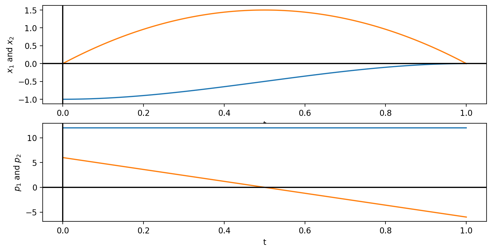
Plots
The routine Flow is not only tensorized but also vectorized, wrt. to tf: when called with a list of final times, the list of corresponding values of the flow are returned (and can be directly used for plotting). For performance reasons, the vectorization is done iteratively: the flow is integrated from t0 to tf[0], then from tf[0] to tf[1] reusing the previous value as initial conditions, and so forth. More on the
vectorize decorator. (See also here for its more advanced use in Flow).
[11]:
N = 100
tspan = list(np.linspace(t0, tf, N+1))
xf, pf = f(t0, x0, p0_sol, tspan, lbda)

fig = plt.figure()
ax1 = fig.add_subplot(211)
ax1.plot(tspan, xf)
ax1.set_xlabel('t')
ax1.set_ylabel('$x_1$ and $x_2$')
ax1.axhline(0, color='k')
ax1.axvline(0, color='k')

ax2 = fig.add_subplot(212)
ax2.plot(tspan, pf)
ax2.set_xlabel('t')
ax2.set_ylabel('$p_1$ and $p_2$')
ax2.axhline(0, color='k')
ax2.axvline(0, color='k')
[11]:
<matplotlib.lines.Line2D at 0x7fd894c423d0>