Notebook source code:
examples/substrate/depletion.ipynb
Run the notebook yourself on binder
![]()
Biomass maximization with substrate depletion
by S. Psalmon and B. Schall (Polytech Nice Sophia, Applied math. dep)

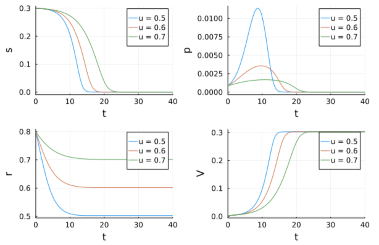
Microorganisms must assign the resources available in their environment to different cellular functions. In nature, it is assumed that bacteria have evolved in a way that their resource allocation strategies maximize their biomass. In our case, the substrate contained in the environment is finite. We define a self-replicator model describing the dynamics of a microbial population growing inside a closed bioreactor of fixed volume. At the beginning of the experience, there is an initial mass of substrate \(S\) inside the bioreactor, that is gradually consumed by the bacterial population. transforming it into precursor metabolites \(P\) building blocks for the creation of proteins and other large molecules. Precursors are transformed into components of the gene expression machinery \(R\) (ribosomes, RNA polymerase etc …), into enzymes that make up the metabolic machinery \(M\), and into a metabolite of interest \(X\) that is excreted from the cell.
While the production of proteins \(M\) and \(R\) is catalyzed by the enzymes \(R\), the absorption of \(S\) and synthesis of X are both catalyzed by \(M\), following these dynamics.
Where \(s\), \(p\), \(r\), \(x\) are the mass fractions of the total bacteria mass of \(S\), \(P\), \(R\) and \(X\), and \(V\) the bacteria’s volume. Here, \(u\) is the allocation control, regulating the production of \(R\) and \(M\). We suppose that compared to \(m\) and \(r\), \(p\) is really small, so we can write \(V = r + m\), that is why \(m\) is not explicit in the system above.
\(w_M\), \(w_R\) and \(w_X\) are function following the Michaelis-Menten kinetics (one of the best-known models of enzyme kinetics), such as :
Where \(K_1,K_2,k_1,k_1\) are constants depending on the bacteria’s environment.
Test of the model with a constant control
[1]:
using DifferentialEquations
using Plots
using JuMP, Ipopt
using Statistics
[2]:
# Giordano et al. (2015)
e_M = 3.6 # 1/h
k_R = 3.6 # 1/h
K_R = 1 # g/L
beta = 0.003 # L/g
# Yegorov et al. (2018)
k_X = 1 # 1/h
K_X = 1 # g/L
k_M = 4.32 #1.2*k_R
K_M = 33.33 #0.1/beta
K = beta*K_R
K_1 = beta*K_X
K_2 = beta*K_M
k_1 = k_X/k_R
k_2 = k_M/k_R
t0 = 0.0 # initial time
tf = 40 # final time
p0 = 0.001 # p0
r0 = 0.8 # r0
V0 = 0.003 # V0
s0= 0.3
Eps = s0+(p0+1)*V0
rmin = r0*(V0/Eps)
rmax = 1-(1-r0)*(V0/Eps)
a=0.5
u0 = [s0, p0, r0, V0]
function derivatives!(du, u, p, t)
s, p, r, V = u
du[1] = (-k_2*s/(K_2+s))*(1-r)*V
du[2] = (k_2*s/(K_2+s))*(1-r) - (p/(K+p))*r*(p+1)
du[3] = (a-r)*(p/(K+p))*r
du[4] = (p/(K+p))*r*V
end
tspan = (0.0, 40.0)
prob5 = ODEProblem(derivatives!,u0,tspan)
alg = RK4()
sol5 = DifferentialEquations.solve(prob5, alg, saveat = 0.01, abstol = 1e-9, reltol = 1e-9)
a = 0.6
prob6 = ODEProblem(derivatives!,u0,tspan)
alg = RK4()
sol6 = DifferentialEquations.solve(prob6, alg, saveat = 0.01, abstol = 1e-9, reltol = 1e-9)
a = 0.7
prob7 = ODEProblem(derivatives!,u0,tspan)
alg = RK4()
sol7 = DifferentialEquations.solve(prob7, alg, saveat = 0.01, abstol = 1e-9, reltol = 1e-9);
[3]:
s = plot(ylabel = "s", fmt = :png)
s = plot!(sol5, vars = 1, label = "u = 0.5")
s = plot!(sol6, vars = 1, label = "u = 0.6")
s = plot!(sol7, vars = 1, label = "u = 0.7")
p = plot(ylabel = "p", fmt = :png)
p = plot!(sol5, vars = 2, label = "u = 0.5")
p = plot!(sol6, vars = 2, label = "u = 0.6")
p = plot!(sol7, vars = 2, label = "u = 0.7")
r = plot(ylabel = "r", fmt = :png)
r = plot!(sol5, vars = 3, label = "u = 0.5")
r = plot!(sol6, vars = 3, label = "u = 0.6")
r = plot!(sol7, vars = 3, label = "u = 0.7")
V = plot(ylabel = "V", fmt = :png)
V = plot!(sol5, vars = 4, label = "u = 0.5")
V = plot!(sol6, vars = 4, label = "u = 0.6")
V = plot!(sol7, vars = 4, label = "u = 0.7")
display(plot(s, p, r, V, layout = (2, 2)))
┌ Warning: To maintain consistency with solution indexing, keyword argument vars will be removed in a future version. Please use keyword argument idxs instead.
│ caller = ip:0x0
└ @ Core :-1

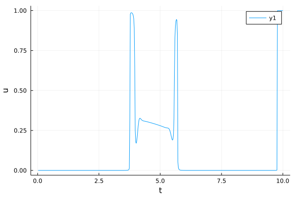
Volume maximisation (no metabolite production)
[4]:
# JuMP model, Ipopt solver
sys = Model(optimizer_with_attributes(Ipopt.Optimizer, "print_level" => 3))
set_optimizer_attribute(sys, "tol", 1e-9)
set_optimizer_attribute(sys, "max_iter", 100000)
# Parameters
# Giordano et al. (2015)
e_M = 3.6 # 1/h
k_R = 3.6 # 1/h
K_R = 1 # g/L
beta = 0.003 # L/g
# Yegorov et al. (2018)
k_X = 1 # 1/h
K_X = 1 # g/L
k_M = 4.32 #1.2*k_R
K_M = 33.33 #0.1/beta
K = beta*K_R
K_1 = beta*K_X
K_2 = beta*K_M
k_1 = k_X/k_R
k_2 = k_M/k_R
t0 = 0.0 # initial time
tf = 10 # final time
p0 = 0.001 # p0
r0 = 0.8 # r0
V0 = 0.01 # V0
s0=0.1
Eps = s0+(p0+1)*V0
rmin = r0*(V0/Eps)
rmax = 1-(1-r0)*(V0/Eps)
N = 500 # grid size
Δt = (tf-t0)/N # Time step
JuMP.@variables(sys, begin
0. ≤ s[1:N] ≤ 1. # s
0. ≤ p[1:N] ≤ 1. # p
rmin ≤ r[1:N] ≤ rmax # r
0. ≤ V[1:N] ≤ Eps # V
0. ≤ u[1:N] ≤ 1. # allocation (control)
end)
# Objective
@objective(sys, Max, V[N])
# Initial conditions
@constraints(sys, begin
s[1] == s0
p[1] == p0
r[1] == r0
V[1] == V0
end)
# Dynamics, Crank-Nicolson scheme
@NLexpression(sys, wR[j = 1:N], p[j]/(K+p[j]))
@NLexpression(sys, wM[j = 1:N], k_2*s[j]/(K_2+s[j]))
for j in 1:N-1
@NLconstraint(sys, # s' = -wM*(1-r)*V
s[j+1] == s[j] + 0.5 * Δt * (-wM[j]*(1-r[j])*V[j] - wM[j+1]*(1-r[j+1])*V[j+1]))
@NLconstraint(sys, # p' = wM*(1-r) - wR*r*(p+1)
p[j+1] == p[j] + 0.5 * Δt * (wM[j]*(1-r[j]) - wR[j]*r[j]*(p[j]+1) + wM[j+1]*(1-r[j+1]) - wR[j+1]*r[j+1]*(p[j+1]+1)))
@NLconstraint(sys, # r' = (u-r)*wR*r
r[j+1] == r[j] + 0.5 * Δt * ((u[j]-r[j])*wR[j]*r[j] + (u[j+1]-r[j+1])*wR[j+1]*r[j+1]))
@NLconstraint(sys, # v' = wR*r*V
V[j+1] == V[j] + 0.5 * Δt * (wR[j]*r[j]*V[j] + wR[j+1]*r[j+1]*V[j+1]))
end
# Solve for the control and state
println("Solving...")
status = optimize!(sys)
println("Solver status: ", status)
p1 = value.(p)
r1 = value.(r)
s1 = value.(s)
V1 = value.(V)
u1 = value.(u)
println("Cost: ", objective_value(sys))
Solving...
******************************************************************************
This program contains Ipopt, a library for large-scale nonlinear optimization.
Ipopt is released as open source code under the Eclipse Public License (EPL).
For more information visit https://github.com/coin-or/Ipopt
******************************************************************************
Total number of variables............................: 2500
variables with only lower bounds: 0
variables with lower and upper bounds: 2500
variables with only upper bounds: 0
Total number of equality constraints.................: 2000
Total number of inequality constraints...............: 0
inequality constraints with only lower bounds: 0
inequality constraints with lower and upper bounds: 0
inequality constraints with only upper bounds: 0
Number of Iterations....: 65
(scaled) (unscaled)
Objective...............: -1.0522150088843175e-01 1.0522150088843175e-01
Dual infeasibility......: 1.2925054411097729e-15 1.2925054411097729e-15
Constraint violation....: 5.9158233867151466e-13 5.9158233867151466e-13
Variable bound violation: 0.0000000000000000e+00 0.0000000000000000e+00
Complementarity.........: 9.0909095584056773e-11 9.0909095584056773e-11
Overall NLP error.......: 9.0909095584056773e-11 9.0909095584056773e-11
Number of objective function evaluations = 79
Number of objective gradient evaluations = 66
Number of equality constraint evaluations = 79
Number of inequality constraint evaluations = 0
Number of equality constraint Jacobian evaluations = 66
Number of inequality constraint Jacobian evaluations = 0
Number of Lagrangian Hessian evaluations = 65
Total seconds in IPOPT = 5.886
EXIT: Optimal Solution Found.
Solver status: nothing
Cost: 0.10522150088843175
[5]:
t = (1:N) * Δt
s_plot = plot(t, s1, xlabel = "t", ylabel = "s", legend = false, fmt = :png)
p_plot = plot(t, p1, xlabel = "t", ylabel = "p", legend = false, fmt = :png)
r_plot = plot(t, r1, xlabel = "t", ylabel = "r", legend = false, fmt = :png)
V_plot = plot(t, V1, xlabel = "t", ylabel = "V", legend = false, fmt = :png)
display(plot(s_plot, p_plot, r_plot, V_plot, layout = (2, 2)))
u_plot = plot(t, u1, xlabel = "t", ylabel = "u", fmt = :png)

[5]:
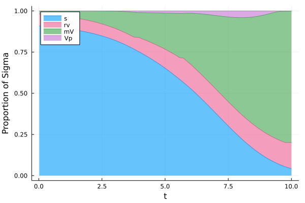
Proportions as a function of time (1/2)
[6]:
y2 = ones(length(s1))
y3 = zeros(length(s1))
plot(t,[s1/Eps (r1.*V1)/Eps+s1/Eps V1/Eps+s1/Eps y2 ] ,xlabel = "t", ylabel = "Proportion of Sigma", fillrange = [y3 s1/Eps s1/Eps+(r1.*V1)/Eps V1/Eps+s1/Eps], fillalpha = 0.6, c = [1 7 3 4] , label = ["s" "rv" "mV" "Vp"], legend = :topleft, fmt = :png)
[6]:
Proportions as a function of time (2/2)
[7]:
@gif for i ∈ 1:(length(t))
pie(["s", "rV", "mV","Vp"], [(s1/Eps)[i], ((r1.*V1)/Eps)[i], ((V1 - (r1.*V1))/Eps)[i],(V1.*p1/Eps)[i]], title = "")
end every 2
┌ Info: Saved animation to
│ fn = /Users/ocots/Boulot/recherche/Logiciels/dev/ct/gallery/examples/substrate/tmp.gif
└ @ Plots /Users/ocots/.julia/packages/Plots/gl4j3/src/animation.jl:137
[7]:

Solution as a function of V0

Solution du problème en fonction du V0 choisi :

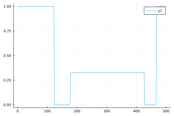
Approximation of solution
[9]:
function approximate(u1)
unull = Array{Float64}(undef, 0)
for i in 1:length(u1)
if 1-10e-3<=u1[i]<= 1
push!(unull, 0)
elseif 0<=u1[i]<= 0+10e-3
push!(unull, 0)
elseif (1-10e-3<=u1[i-1]<= 1 && 0<=u1[i+1]<= 0+10e-3) || (1-10e-3<=u1[i+1]<= 1 && 0<=u1[i-1]<= 0+10e-3)
push!(unull, 0)
else
push!(unull, u1[i])
end
end
indexes = Vector{Int64}(undef, 0)
for i in 1:length(unull)
if unull[i] != 0
push!(indexes, i)
end
end
y = u1[indexes[1]:indexes[length(indexes)]]
m = mean(y)
m_array = m*ones(length(y),1)
t = LinRange(0, tf, length(u1))
plot(t,vcat(u1[1:indexes[1]-1],m_array,u1[indexes[length(indexes)]+1:length(unull)]),fmt = :png)
return vcat(u1[1:indexes[1]-1],m_array,u1[indexes[length(indexes)]+1:length(unull)])
end;
[10]:
# JuMP model, Ipopt solver
sys = Model(optimizer_with_attributes(Ipopt.Optimizer, "print_level" => 3))
set_optimizer_attribute(sys, "tol", 1e-9)
set_optimizer_attribute(sys, "max_iter", 100000)
# Parameters
# Giordano et al. (2015)
e_M = 3.6 # 1/h
k_R = 3.6 # 1/h
K_R = 1 # g/L
beta = 0.003 # L/g
# Yegorov et al. (2018)
k_X = 1 # 1/h
K_X = 1 # g/L
k_M = 4.32 #1.2*k_R
K_M = 33.33 #0.1/beta
K = beta*K_R
K_1 = beta*K_X
K_2 = beta*K_M
k_1 = k_X/k_R
k_2 = k_M/k_R
t0 = 0.0 # initial time
tf = 10 # final time
p0 = 0.003 # p0
r0 = 0.1 # r0
V0 = 0.003 # V0
s0=0.1
Eps = s0+(p0+1)*V0
rmin = r0*(V0/Eps)
rmax = 1-(1-r0)*(V0/Eps)
N = 500 # grid size
Δt = (tf-t0)/N # Time step
JuMP.@variables(sys, begin
0. ≤ s[1:N] ≤ 1. # s
0. ≤ p[1:N] ≤ 1. # p
rmin ≤ r[1:N] ≤ rmax # r
0. ≤ V[1:N] ≤ Eps # V
0. ≤ u[1:N] ≤ 1. # allocation (control)
end)
# Objective
@objective(sys, Max, V[N])
# Initial conditions
@constraints(sys, begin
s[1] == s0
p[1] == p0
r[1] == r0
V[1] == V0
end)
# Dynamics, Crank-Nicolson scheme
@NLexpression(sys, wR[j = 1:N], p[j]/(K+p[j]))
@NLexpression(sys, wM[j = 1:N], k_2*s[j]/(K_2+s[j]))
for j in 1:N-1
@NLconstraint(sys, # s' = -wM*(1-r)*V
s[j+1] == s[j] + 0.5 * Δt * (-wM[j]*(1-r[j])*V[j] - wM[j+1]*(1-r[j+1])*V[j+1]))
@NLconstraint(sys, # p' = wM*(1-r) - wR*r*(p+1)
p[j+1] == p[j] + 0.5 * Δt * (wM[j]*(1-r[j]) - wR[j]*r[j]*(p[j]+1) + wM[j+1]*(1-r[j+1]) - wR[j+1]*r[j+1]*(p[j+1]+1)))
@NLconstraint(sys, # r' = (u-r)*wR*r
r[j+1] == r[j] + 0.5 * Δt * ((u[j]-r[j])*wR[j]*r[j] + (u[j+1]-r[j+1])*wR[j+1]*r[j+1]))
@NLconstraint(sys, # v' = wR*r*V
V[j+1] == V[j] + 0.5 * Δt * (wR[j]*r[j]*V[j] + wR[j+1]*r[j+1]*V[j+1]))
end
# Solve for the control and state
println("Solving...")
status = optimize!(sys)
println("Solver status: ", status)
p1 = value.(p)
r1 = value.(r)
s1 = value.(s)
V1 = value.(V)
u1 = value.(u)
println("Cost: ", objective_value(sys))
u_appr = approximate(u1)
plot(u_appr, fmt = :png)
Solving...
Total number of variables............................: 2500
variables with only lower bounds: 0
variables with lower and upper bounds: 2500
variables with only upper bounds: 0
Total number of equality constraints.................: 2000
Total number of inequality constraints...............: 0
inequality constraints with only lower bounds: 0
inequality constraints with lower and upper bounds: 0
inequality constraints with only upper bounds: 0
Number of Iterations....: 39
(scaled) (unscaled)
Objective...............: -7.0297356929830648e-02 7.0297356929830648e-02
Dual infeasibility......: 1.7903724391439148e-13 1.7903724391439148e-13
Constraint violation....: 3.9059477874303639e-11 3.9059477874303639e-11
Variable bound violation: 0.0000000000000000e+00 0.0000000000000000e+00
Complementarity.........: 9.0911737904302616e-11 9.0911737904302616e-11
Overall NLP error.......: 9.0911737904302616e-11 9.0911737904302616e-11
Number of objective function evaluations = 40
Number of objective gradient evaluations = 40
Number of equality constraint evaluations = 40
Number of inequality constraint evaluations = 0
Number of equality constraint Jacobian evaluations = 40
Number of inequality constraint Jacobian evaluations = 0
Number of Lagrangian Hessian evaluations = 39
Total seconds in IPOPT = 1.033
EXIT: Optimal Solution Found.
Solver status: nothing
Cost: 0.07029735692983065
[10]:
Testing the approximation
[11]:
# JuMP model, Ipopt solver
sys = Model(optimizer_with_attributes(Ipopt.Optimizer, "print_level" => 3))
set_optimizer_attribute(sys, "tol", 1e-9)
set_optimizer_attribute(sys, "max_iter", 100000)
# Parameters
# Giordano et al. (2015)
e_M = 3.6 # 1/h
k_R = 3.6 # 1/h
K_R = 1 # g/L
beta = 0.003 # L/g
# Yegorov et al. (2018)
k_X = 1 # 1/h
K_X = 1 # g/L
k_M = 4.32 #1.2*k_R
K_M = 33.33 #0.1/beta
K = beta*K_R
K_1 = beta*K_X
K_2 = beta*K_M
k_1 = k_X/k_R
k_2 = k_M/k_R
t0 = 0.0 # initial time
tf = 10 # final time
p0 = 0.003 # p0
r0 = 0.1 # r0
V0 = 0.003 # V0
s0=0.1
Eps = s0+(p0+1)*V0
rmin = r0*(V0/Eps)
rmax = 1-(1-r0)*(V0/Eps)
N = 500 # grid size
Δt = (tf-t0)/N # Time step
JuMP.@variables(sys, begin
0. ≤ s[1:N] ≤ 1. # s
0. ≤ p[1:N] ≤ 1. # p
rmin ≤ r[1:N] ≤ rmax # r
0. ≤ V[1:N] ≤ Eps # V
0. ≤ u[1:N] ≤ 1. # allocation (control)
end)
# Objective
@objective(sys, Max, V[N])
# Initial conditions
@constraints(sys, begin
s[1] == s0
p[1] == p0
r[1] == r0
V[1] == V0
u[1] == u_appr[1]
end)
# Dynamics, Crank-Nicolson scheme
@NLexpression(sys, wR[j = 1:N], p[j]/(K+p[j]))
@NLexpression(sys, wM[j = 1:N], k_2*s[j]/(K_2+s[j]))
for j in 1:N-1
@NLconstraint(sys, # s' = -wM*(1-r)*V
s[j+1] == s[j] + 0.5 * Δt * (-wM[j]*(1-r[j])*V[j] - wM[j+1]*(1-r[j+1])*V[j+1]))
@NLconstraint(sys, # p' = wM*(1-r) - wR*r*(p+1)
p[j+1] == p[j] + 0.5 * Δt * (wM[j]*(1-r[j]) - wR[j]*r[j]*(p[j]+1) + wM[j+1]*(1-r[j+1]) - wR[j+1]*r[j+1]*(p[j+1]+1)))
@NLconstraint(sys, # r' = (u-r)*wR*r
r[j+1] == r[j] + 0.5 * Δt * ((u[j]-r[j])*wR[j]*r[j] + (u[j+1]-r[j+1])*wR[j+1]*r[j+1]))
@NLconstraint(sys, # v' = wR*r*V
V[j+1] == V[j] + 0.5 * Δt * (wR[j]*r[j]*V[j] + wR[j+1]*r[j+1]*V[j+1]))
@NLconstraint(sys, # v' = wR*r*V
u[j+1] == u_appr[j+1])
end
# Solve for the control and state
println("Solving...")
status = optimize!(sys)
println("Solver status: ", status)
p2 = value.(p)
r2 = value.(r)
s2 = value.(s)
V2 = value.(V)
u2 = value.(u)
println("Cost: ", objective_value(sys))
Solving...
Total number of variables............................: 2500
variables with only lower bounds: 0
variables with lower and upper bounds: 2500
variables with only upper bounds: 0
Total number of equality constraints.................: 2500
Total number of inequality constraints...............: 0
inequality constraints with only lower bounds: 0
inequality constraints with lower and upper bounds: 0
inequality constraints with only upper bounds: 0
Number of Iterations....: 11
(scaled) (unscaled)
Objective...............: -6.9578730588867710e-02 6.9578730588867710e-02
Dual infeasibility......: 1.5666602130176566e-13 1.5666602130176566e-13
Constraint violation....: 1.0016016575159492e-10 1.0016016575159492e-10
Variable bound violation: 0.0000000000000000e+00 0.0000000000000000e+00
Complementarity.........: 0.0000000000000000e+00 0.0000000000000000e+00
Overall NLP error.......: 1.0016016575159492e-10 1.0016016575159492e-10
Number of objective function evaluations = 12
Number of objective gradient evaluations = 12
Number of equality constraint evaluations = 12
Number of inequality constraint evaluations = 0
Number of equality constraint Jacobian evaluations = 12
Number of inequality constraint Jacobian evaluations = 0
Number of Lagrangian Hessian evaluations = 11
Total seconds in IPOPT = 0.302
EXIT: Optimal Solution Found.
Solver status: nothing
Cost: 0.06957873058886771
[12]:
# Plots
t = (1:N) * Δt
s_plot = plot(t, s2, xlabel = "t", ylabel = "s", legend = false, fmt = :png)
p_plot = plot(t, p2, xlabel = "t", ylabel = "p", legend = false, fmt = :png)
r_plot = plot(t, r2, xlabel = "t", ylabel = "r", legend = false, fmt = :png)
V_plot = plot(t, V2, xlabel = "t", ylabel = "V", legend = false, fmt = :png)
display(plot(s_plot, p_plot, r_plot, V_plot, layout = (2, 2)))
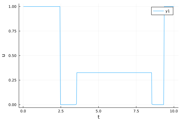
u_plot = plot(t, u2, xlabel = "t", ylabel = "u", fmt = :png)

[12]:
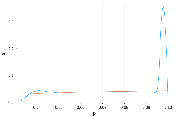
Singular arc plot
[13]:
function p_func(s)
return sqrt(K*(k_2*s)/(K_2+s))
end
sp_plot = plot(s1, [p1, p_func], xlabel = "p", ylabel = "s", legend = false, fmt = :png)
[13]:
Metabolite production maximisation
[14]:
# JuMP model, Ipopt solver
sys = Model(optimizer_with_attributes(Ipopt.Optimizer, "print_level" => 3))
set_optimizer_attribute(sys, "tol", 1e-12)
# Parameters
k_r = 3.6
k_m = 4.32
k_x = 0.5
K_r = 1
K_m = 33.3
K_x = 1
Beta = 0.003
K = Beta*K_r
K_1 = Beta*K_x
K_2 = Beta*K_m
k_1 = k_x/k_r
k_2 = k_m/k_r
t0 = 0.0 # initial time
tf = 14 # final time
p0 = 0.001 # p0
r0 = 0.8 # r0
V0 = 0.003 # V0
x0 = 0
s0 = 0.3
Eps = s0+(p0+1)*V0
rmin = r0*(V0/Eps)
rmax = 1-(1-r0)*(V0/Eps)
N = 500 # grid size
Δt = (tf-t0)/N # Time step
JuMP.@variables(sys, begin
0. ≤ s[1:N] ≤ 1. # s
0. ≤ p[1:N] ≤ 1. # p
rmin ≤ r[1:N] ≤ rmax # r
0. ≤ V[1:N] ≤ Eps # V
0. ≤ u[1:N] ≤ 1. # allocation (control)
0. ≤ x[1:N] ≤ Eps-V0
end)
# Objective
@objective(sys, Max, x[N])
# Initial conditions
@constraints(sys, begin
s[1] == s0
p[1] == p0
r[1] == r0
V[1] == V0
x[1] == x0
end)
# Dynamics, Crank-Nicolson scheme
@NLexpression(sys, wR[j = 1:N], p[j]/(K+p[j]))
@NLexpression(sys, wM[j = 1:N], k_2*s[j]/(K_2+s[j]))
@NLexpression(sys, wX[j = 1:N], k_1*p[j]/(K_1+p[j]))
for j in 1:N-1
@NLconstraint(sys, # s' = -wM*(1-r)*V
s[j+1] == s[j] + 0.5 * Δt * (-wM[j]*(1-r[j])*V[j] - wM[j+1]*(1-r[j+1])*V[j+1]))
@NLconstraint(sys, # p' = wM*(1-r) - wR*r*(p+1)
p[j+1] == p[j] + 0.5 * Δt * (wM[j]*(1-r[j]) - wR[j]*r[j]*(p[j]+1) - wX[j]*(1-r[j]) + wM[j+1]*(1-r[j+1]) - wR[j+1]*r[j+1]*(p[j+1]+1) - wX[j+1]*(1-r[j+1])))
@NLconstraint(sys, # r' = (u-r)*wR*r
r[j+1] == r[j] + 0.5 * Δt * ((u[j]-r[j])*wR[j]*r[j] + (u[j+1]-r[j+1])*wR[j+1]*r[j+1]))
@NLconstraint(sys, # v' = wR*r*V
V[j+1] == V[j] + 0.5 * Δt * (wR[j]*r[j]*V[j] + wR[j+1]*r[j+1]*V[j+1]))
@NLconstraint(sys, # x' = wX*(1-r)*V
x[j+1] == x[j] + 0.5 * Δt * (wX[j]*(1-r[j])*V[j] + wX[j+1]*(1-r[j+1])*V[j+1]))
end
# Solve for the control and state
println("Solving...")
status = optimize!(sys)
println("Solver status: ", status)
p1 = value.(p)
r1 = value.(r)
s1 = value.(s)
V1 = value.(V)
x1 = value.(x)
u1 = value.(u)
println("Cost: ", objective_value(sys))
Solving...
Total number of variables............................: 3000
variables with only lower bounds: 0
variables with lower and upper bounds: 3000
variables with only upper bounds: 0
Total number of equality constraints.................: 2500
Total number of inequality constraints...............: 0
inequality constraints with only lower bounds: 0
inequality constraints with lower and upper bounds: 0
inequality constraints with only upper bounds: 0
Number of Iterations....: 43
(scaled) (unscaled)
Objective...............: -9.8033649328755273e-02 9.8033649328755273e-02
Dual infeasibility......: 3.9257501258990043e-15 3.9257501258990043e-15
Constraint violation....: 1.9428902930940239e-15 1.9428902930940239e-15
Variable bound violation: 9.5934357146388206e-09 9.5934357146388206e-09
Complementarity.........: 1.2544302998615077e-13 1.2544302998615077e-13
Overall NLP error.......: 1.2544302998615077e-13 1.2544302998615077e-13
Number of objective function evaluations = 44
Number of objective gradient evaluations = 44
Number of equality constraint evaluations = 44
Number of inequality constraint evaluations = 0
Number of equality constraint Jacobian evaluations = 44
Number of inequality constraint Jacobian evaluations = 0
Number of Lagrangian Hessian evaluations = 43
Total seconds in IPOPT = 1.491
EXIT: Optimal Solution Found.
Solver status: nothing
Cost: 0.09803364932875527
[15]:
# Plots
t = (1:N) * Δt
s_plot = plot(t, s1, xlabel = "t", ylabel = "s", legend = false, fmt = :png)
p_plot = plot(t, p1, xlabel = "t", ylabel = "p", legend = false, fmt = :png)
r_plot = plot(t, r1, xlabel = "t", ylabel = "r", legend = false, fmt = :png)
V_plot = plot(t, V1, xlabel = "t", ylabel = "V", legend = false, fmt = :png)
x_plot = plot(t, x1, xlabel = "t", ylabel = "x", legend = false, fmt = :png)
u_plot = plot(t, u1, xlabel = "t", ylabel = "u", legend = false, fmt = :png)
display(plot(s_plot, p_plot, r_plot, V_plot, x_plot, u_plot, layout = (3, 2)))

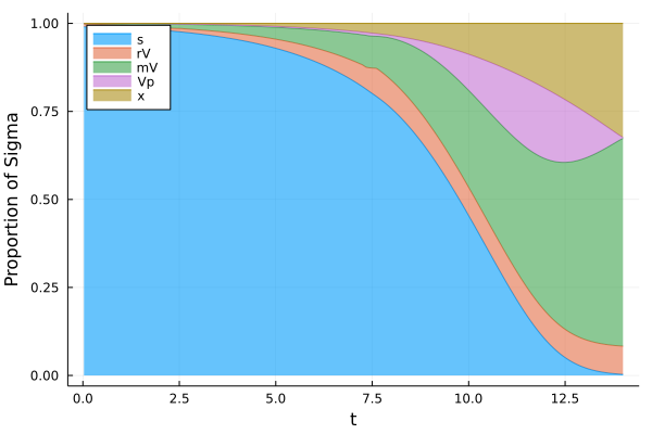
Proportions as a function of time (1/2)
[16]:
y2 = ones(length(s1))
y3 = zeros(length(s1))
plot(t,[s1/Eps (r1.*V1)/Eps+s1/Eps V1/Eps+s1/Eps V1/Eps+s1/Eps+(V1.*p1)/Eps y2 ] ,xlabel = "t", ylabel = "Proportion of Sigma", fillrange = [y3 s1/Eps (r1.*V1)/Eps+s1/Eps s1/Eps+V1/Eps V1/Eps+s1/Eps+(V1.*p1)/Eps], fillalpha = 0.6, c = [1 2 3 4 5] , label = ["s" "rV" "mV" "Vp" "x"], legend = :topleft, fmt = :png)
[16]:
Proportions as a function of time (2/2)
[17]:
@gif for i ∈ 1:(length(t))
pie(["s", "rV", "mV","Vp","x"], [(s1/Eps)[i], ((r1.*V1)/Eps)[i], ((V1 - (r1.*V1))/Eps)[i],(V1.*p1/Eps)[i], (x1/Eps)[i]])
end every 1
┌ Info: Saved animation to
│ fn = /Users/ocots/Boulot/recherche/Logiciels/dev/ct/gallery/examples/substrate/tmp.gif
└ @ Plots /Users/ocots/.julia/packages/Plots/gl4j3/src/animation.jl:137
[17]:

Volume maximisation with metabolite production
[18]:
# JuMP model, Ipopt solver
sys = Model(optimizer_with_attributes(Ipopt.Optimizer, "print_level" => 3))
set_optimizer_attribute(sys, "tol", 1e-12)
# Parameters
k_r = 3.6
k_m = 4.32
k_x = 0.5
K_r = 1
K_m = 33.3
K_x = 1
Beta = 0.003
K = Beta*K_r
K_1 = Beta*K_x
K_2 = Beta*K_m
k_1 = k_x/k_r
k_2 = k_m/k_r
t0 = 0.0 # initial time
tf = 20 # final time
p0 = 0.001 # p0
r0 = 0.8 # r0
V0 = 0.003 # V0
x0 = 0
s0 = 0.3
Eps = s0+(p0+1)*V0+x0
rmin = r0*(V0/Eps)
rmax = 1-(1-r0)*(V0/Eps)
N = 1000 # grid size
Δt = (tf-t0)/N # Time step
JuMP.@variables(sys, begin
0. ≤ s[1:N] ≤ 1. # s
0. ≤ p[1:N] ≤ 1. # p
rmin ≤ r[1:N] ≤ rmax # r
0. ≤ V[1:N] ≤ Eps # V
0. ≤ u[1:N] ≤ 1. # allocation (control)
0. ≤ x[1:N] ≤ Eps-V0
end)
# Objective
@objective(sys, Max, V[N])
# Initial conditions
@constraints(sys, begin
s[1] == s0
p[1] == p0
r[1] == r0
V[1] == V0
x[1] == x0
end)
# Dynamics, Crank-Nicolson scheme
@NLexpression(sys, wR[j = 1:N], p[j]/(K+p[j]))
@NLexpression(sys, wM[j = 1:N], k_2*s[j]/(K_2+s[j]))
@NLexpression(sys, wX[j = 1:N], k_1*p[j]/(K_1+p[j]))
for j in 1:N-1
@NLconstraint(sys, # s' = -wM*(1-r)*V
s[j+1] == s[j] + 0.5 * Δt * (-wM[j]*(1-r[j])*V[j] - wM[j+1]*(1-r[j+1])*V[j+1]))
@NLconstraint(sys, # p' = wM*(1-r) - wR*r*(p+1)
p[j+1] == p[j] + 0.5 * Δt * (wM[j]*(1-r[j]) - wR[j]*r[j]*(p[j]+1) - wX[j]*(1-r[j]) + wM[j+1]*(1-r[j+1]) - wR[j+1]*r[j+1]*(p[j+1]+1) - wX[j+1]*(1-r[j+1])))
@NLconstraint(sys, # r' = (u-r)*wR*r
r[j+1] == r[j] + 0.5 * Δt * ((u[j]-r[j])*wR[j]*r[j] + (u[j+1]-r[j+1])*wR[j+1]*r[j+1]))
@NLconstraint(sys, # v' = wR*r*V
V[j+1] == V[j] + 0.5 * Δt * (wR[j]*r[j]*V[j] + wR[j+1]*r[j+1]*V[j+1]))
@NLconstraint(sys, # x' = wX*(1-r)*V
x[j+1] == x[j] + 0.5 * Δt * (wX[j]*(1-r[j])*V[j] + wX[j+1]*(1-r[j+1])*V[j+1]))
end
# Solve for the control and state
println("Solving...")
status = optimize!(sys)
println("Solver status: ", status)
p2 = value.(p)
r2= value.(r)
s2 = value.(s)
V2 = value.(V)
x2 = value.(x)
u2 = value.(u)
println("Cost: ", objective_value(sys))
Solving...
Total number of variables............................: 6000
variables with only lower bounds: 0
variables with lower and upper bounds: 6000
variables with only upper bounds: 0
Total number of equality constraints.................: 5000
Total number of inequality constraints...............: 0
inequality constraints with only lower bounds: 0
inequality constraints with lower and upper bounds: 0
inequality constraints with only upper bounds: 0
Number of Iterations....: 1208
(scaled) (unscaled)
Objective...............: -2.8358279561639799e-01 2.8358279561639799e-01
Dual infeasibility......: 1.0099687300350739e-15 1.0099687300350739e-15
Constraint violation....: 4.7184478546569153e-15 4.7184478546569153e-15
Variable bound violation: 4.0786095372712861e-09 4.0786095372712861e-09
Complementarity.........: 1.2544303607314760e-13 1.2544303607314760e-13
Overall NLP error.......: 1.2544303607314760e-13 1.2544303607314760e-13
Number of objective function evaluations = 1921
Number of objective gradient evaluations = 1201
Number of equality constraint evaluations = 1921
Number of inequality constraint evaluations = 0
Number of equality constraint Jacobian evaluations = 1218
Number of inequality constraint Jacobian evaluations = 0
Number of Lagrangian Hessian evaluations = 1208
Total seconds in IPOPT = 90.764
EXIT: Optimal Solution Found.
Solver status: nothing
Cost: 0.283582795616398
[19]:
# Plots
t = (1:N) * Δt
s_plot = plot(t, s2, xlabel = "t", ylabel = "s", legend = false, fmt = :png)
p_plot = plot(t, p2, xlabel = "t", ylabel = "p", legend = false, fmt = :png)
r_plot = plot(t, r2, xlabel = "t", ylabel = "r", legend = false, fmt = :png)
V_plot = plot(t, V2, xlabel = "t", ylabel = "V", legend = false, fmt = :png)
x_plot = plot(t, x2, xlabel = "t", ylabel = "x", legend = false, fmt = :png)
u_plot = plot(t, u2, xlabel = "t", ylabel = "u", legend = false, fmt = :png)
display(plot(s_plot, p_plot, r_plot, V_plot, x_plot, u_plot, layout = (3, 2)))

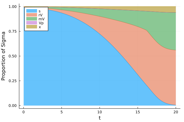
Proportions as a function of time (1/2)
[20]:
y2 = ones(length(s2))
y3 = zeros(length(s2))
plot(t,[s2/Eps (r2.*V2)/Eps+s2/Eps V2/Eps+s2/Eps V2/Eps+s2/Eps+(V2.*p2)/Eps y2 ] ,xlabel = "t", ylabel = "Proportion of Sigma", fillrange = [y3 s2/Eps (r2.*V2)/Eps+s2/Eps s2/Eps+V2/Eps V2/Eps+s2/Eps+(V2.*p2)/Eps], fillalpha = 0.6, c = [1 2 3 4 5] , label = ["s" "rV" "mV" "Vp" "x"], legend = :topleft, fmt = :png)
[20]:
Proportions as a function of time (2/2)
[21]:
@gif for i ∈ 1:(length(t))
pie(["s", "rV", "mV","Vp","x"], [(s2/Eps)[i], ((r2.*V2)/Eps)[i], ((V2 - (r2.*V2))/Eps)[i],(V2.*p2/Eps)[i], (x2/Eps)[i]])
end every 1
┌ Info: Saved animation to
│ fn = /Users/ocots/Boulot/recherche/Logiciels/dev/ct/gallery/examples/substrate/tmp.gif
└ @ Plots /Users/ocots/.julia/packages/Plots/gl4j3/src/animation.jl:137
[21]:

Time minimisation under fixed performance (final volume)
[22]:
# JuMP model, Ipopt solver
sys = Model(optimizer_with_attributes(Ipopt.Optimizer, "print_level" => 5))
set_optimizer_attribute(sys, "tol", 1e-12)
set_optimizer_attribute(sys, "max_iter", 1000)
# Parameters
# Giordano et al. (2015)
e_M = 3.6 # 1/h
k_R = 3.6 # 1/h
K_R = 1 # g/L
beta = 0.003 # L/g
# Yegorov et al. (2018)
k_X = 1 # 1/h
K_X = 1 # g/L
k_M = 4.32 #1.2*k_R
K_M = 33.33 #0.1/beta
K = beta*K_R
K_1 = beta*K_X
K_2 = beta*K_M
k_1 = k_X/k_R
k_2 = k_M/k_R
t0 = 0.0 # initial time
tf = 40 # final time
p0 = 0.003 # p0
r0 = 0.1 # r0
V0 = 0.003 # V0
s0=0.1
eta = 0.90
Eps = s0+(p0+1)*V0
rmin = r0*(V0/Eps)
rmax = 1-(1-r0)*(V0/Eps)
N = 500 # grid size
JuMP.@variables(sys, begin
0. ≤ s[1:N] ≤ 1. # s
0. ≤ p[1:N] ≤ 1. # p
rmin ≤ r[1:N] ≤ rmax # r
0. ≤ V[1:N] ≤ eta*Eps # V
0. ≤ u[1:N] ≤ 1.
0. ≤ Δt[1] ≤ 1.
end)
# Objective
@objective(sys, Min, Δt[1])
# Initial conditions
@constraints(sys, begin
s[1] == s0
p[1] == p0
r[1] == r0
V[1] == V0
V[N] == eta*Eps
end)
# Dynamics, Crank-Nicolson scheme
@NLexpression(sys, wR[j = 1:N], p[j]/(K+p[j]))
@NLexpression(sys, wM[j = 1:N], k_2*s[j]/(K_2+s[j]))
for j in 1:N-1
@NLconstraint(sys, # s' = -wM*(1-r)*V
s[j+1] == s[j] + 0.5 * Δt[1] * (-wM[j]*(1-r[j])*V[j] - wM[j+1]*(1-r[j+1])*V[j+1]))
@NLconstraint(sys, # p' = wM*(1-r) - wR*r*(p+1)
p[j+1] == p[j] + 0.5 * Δt[1] * (wM[j]*(1-r[j]) - wR[j]*r[j]*(p[j]+1) + wM[j+1]*(1-r[j+1]) - wR[j+1]*r[j+1]*(p[j+1]+1)))
@NLconstraint(sys, # r' = (u-r)*wR*r
r[j+1] == r[j] + 0.5 * Δt[1] * ((u[j]-r[j])*wR[j]*r[j] + (u[j+1]-r[j+1])*wR[j+1]*r[j+1]))
@NLconstraint(sys, # v' = wR*r*V
V[j+1] == V[j] + 0.5 * Δt[1] * (wR[j]*r[j]*V[j] + wR[j+1]*r[j+1]*V[j+1]))
end
# Solve for the control and state
println("Solving...")
status = optimize!(sys)
println("Solver status: ", status)
p1 = value.(p)
r1 = value.(r)
s1 = value.(s)
V1 = value.(V)
u1 = value.(u)
println("Cost: ", objective_value(sys))
┌ Warning: Axis contains one element: 1. If intended, you can safely ignore this warning. To explicitly pass the axis with one element, pass `[1]` instead of `1`.
└ @ JuMP.Containers /Users/ocots/.julia/packages/JuMP/UqjgA/src/Containers/DenseAxisArray.jl:173
Solving...
This is Ipopt version 3.14.4, running with linear solver MUMPS 5.4.1.
Number of nonzeros in equality constraint Jacobian...: 13977
Number of nonzeros in inequality constraint Jacobian.: 0
Number of nonzeros in Lagrangian Hessian.............: 55888
Total number of variables............................: 2501
variables with only lower bounds: 0
variables with lower and upper bounds: 2501
variables with only upper bounds: 0
Total number of equality constraints.................: 2001
Total number of inequality constraints...............: 0
inequality constraints with only lower bounds: 0
inequality constraints with lower and upper bounds: 0
inequality constraints with only upper bounds: 0
iter objective inf_pr inf_du lg(mu) ||d|| lg(rg) alpha_du alpha_pr ls
0 9.9999900e-03 9.18e-02 8.40e-06 -1.0 0.00e+00 - 0.00e+00 0.00e+00 0
1 4.4500801e-02 9.10e-02 1.73e+05 -1.7 1.11e+02 - 8.90e-05 8.81e-03f 1
2 4.5510331e-02 9.09e-02 1.72e+05 -1.7 2.49e+02 - 1.65e-04 3.11e-04f 1
3 5.1510453e-02 9.07e-02 1.42e+05 -1.7 3.84e+01 2.0 1.88e-04 2.85e-03h 1
4 5.1752183e-02 9.07e-02 1.42e+05 -1.7 4.48e+01 1.5 3.66e-04 1.19e-04h 1
5 5.1819771e-02 9.07e-02 1.42e+05 -1.7 8.65e+01 1.0 3.23e-05 3.46e-05h 1
6 5.1822782e-02 9.07e-02 1.42e+05 -1.7 2.81e+02 0.6 2.11e-06 1.52e-06f 2
7 5.1856808e-02 9.07e-02 1.42e+05 -1.7 9.53e+01 1.0 1.30e-05 1.75e-05h 1
8 5.1881279e-02 9.07e-02 1.42e+05 -1.7 3.41e+02 0.5 7.48e-07 1.23e-05f 1
9 5.1881626e-02 9.07e-02 1.42e+05 -1.7 9.99e+01 0.9 1.52e-06 1.82e-07f 4
iter objective inf_pr inf_du lg(mu) ||d|| lg(rg) alpha_du alpha_pr ls
10 5.1903040e-02 9.07e-02 1.42e+05 -1.7 4.17e+02 0.5 5.23e-07 1.07e-05f 1
11r 5.1903040e-02 9.07e-02 9.99e+02 -1.0 0.00e+00 0.9 0.00e+00 2.72e-07R 3
12r 5.0910260e-02 9.05e-02 9.98e+02 -1.0 1.57e+00 - 2.92e-05 1.26e-03f 1
13r 3.8167861e-02 8.86e-02 9.81e+02 -1.0 9.86e-01 - 1.99e-02 1.67e-02f 1
14r 2.7444055e-02 8.59e-02 9.60e+02 -1.0 6.52e-01 - 2.40e-02 2.15e-02f 1
15r 1.4356924e-02 7.94e-02 9.87e+02 -1.0 4.05e-01 - 2.20e-02 4.81e-02f 1
16 1.5652546e-02 7.89e-02 6.31e+02 -1.7 6.44e+00 - 3.33e-03 6.95e-03h 1
17 1.5810028e-02 7.88e-02 6.42e+02 -1.7 2.86e+01 - 1.45e-03 8.24e-04h 1
18 1.6014058e-02 7.87e-02 6.56e+02 -1.7 2.78e+01 - 8.01e-04 1.10e-03f 1
19 1.6173077e-02 7.87e-02 6.62e+02 -1.7 2.45e+01 - 9.09e-05 8.84e-04f 1
iter objective inf_pr inf_du lg(mu) ||d|| lg(rg) alpha_du alpha_pr ls
20 1.6330161e-02 7.86e-02 6.67e+02 -1.7 2.28e+01 - 1.26e-04 8.81e-04f 1
21 1.6480098e-02 7.85e-02 6.70e+02 -1.7 2.09e+01 - 1.62e-04 8.48e-04f 1
22 1.6625105e-02 7.85e-02 6.73e+02 -1.7 1.88e+01 - 1.71e-04 8.26e-04h 1
23 1.6764922e-02 7.84e-02 6.75e+02 -1.7 1.66e+01 - 1.59e-04 8.03e-04h 1
24 1.6896131e-02 7.83e-02 6.76e+02 -1.7 1.48e+01 - 1.32e-04 7.61e-04h 1
25 1.6912599e-02 7.83e-02 6.76e+02 -1.7 1.40e+01 - 9.23e-05 9.62e-05h 1
26 1.7000587e-02 7.83e-02 6.77e+02 -1.7 1.21e+01 - 9.44e-04 5.25e-04h 1
27 1.7104795e-02 7.83e-02 6.77e+02 -1.7 1.05e+01 - 2.58e-04 6.34e-04h 1
28 1.7203516e-02 7.82e-02 6.78e+02 -1.7 9.88e+00 - 3.51e-04 6.05e-04h 1
29 1.7298454e-02 7.82e-02 6.78e+02 -1.7 9.23e+00 - 8.46e-05 5.86e-04h 1
iter objective inf_pr inf_du lg(mu) ||d|| lg(rg) alpha_du alpha_pr ls
30 1.7398237e-02 7.81e-02 6.78e+02 -1.7 9.40e+00 - 6.13e-05 6.14e-04h 1
31 1.7400818e-02 7.81e-02 6.78e+02 -1.7 1.08e+01 - 3.03e-05 1.56e-05h 1
32 1.7492996e-02 7.81e-02 6.78e+02 -1.7 7.68e+00 - 2.82e-04 5.81e-04f 1
33 1.7602310e-02 7.80e-02 6.78e+02 -1.7 7.76e+00 - 3.12e-04 6.89e-04h 1
34 1.7697095e-02 7.80e-02 6.78e+02 -1.7 7.40e+00 - 1.05e-04 6.01e-04h 1
35 1.7797276e-02 7.79e-02 6.78e+02 -1.7 7.52e+00 - 6.70e-05 6.34e-04h 1
36 1.7800504e-02 7.79e-02 6.78e+02 -1.7 8.39e+00 - 3.56e-05 2.01e-05h 1
37 1.7895873e-02 7.79e-02 6.78e+02 -1.7 6.34e+00 - 3.90e-04 6.15e-04f 1
38 1.8006477e-02 7.78e-02 6.78e+02 -1.7 6.27e+00 - 3.32e-04 7.15e-04h 1
39 1.8105211e-02 7.78e-02 6.78e+02 -1.7 5.98e+00 - 2.53e-04 6.42e-04h 1
iter objective inf_pr inf_du lg(mu) ||d|| lg(rg) alpha_du alpha_pr ls
40 1.8206404e-02 7.77e-02 6.78e+02 -1.7 5.88e+00 - 8.29e-05 6.59e-04h 1
41 1.8258537e-02 7.77e-02 6.78e+02 -1.7 6.08e+00 - 6.31e-05 3.39e-04h 1
42 1.8309806e-02 7.77e-02 6.77e+02 -1.7 5.41e+00 - 3.54e-04 3.37e-04f 1
43 1.8417214e-02 7.76e-02 6.77e+02 -1.7 5.26e+00 - 1.73e-04 7.13e-04f 1
44 1.8527105e-02 7.75e-02 6.77e+02 -1.7 5.27e+00 - 3.45e-04 7.30e-04h 1
45 1.8633348e-02 7.75e-02 6.77e+02 -1.7 5.17e+00 - 2.85e-04 7.10e-04h 1
46 1.8741984e-02 7.74e-02 6.76e+02 -1.7 5.08e+00 - 2.63e-04 7.30e-04h 1
47 1.8852667e-02 7.74e-02 6.76e+02 -1.7 5.00e+00 - 2.60e-04 7.47e-04h 1
48 1.8965183e-02 7.73e-02 6.75e+02 -1.7 4.92e+00 - 2.60e-04 7.63e-04h 1
49 1.9079703e-02 7.73e-02 6.75e+02 -1.7 4.84e+00 - 2.61e-04 7.81e-04h 1
iter objective inf_pr inf_du lg(mu) ||d|| lg(rg) alpha_du alpha_pr ls
50 1.9196344e-02 7.72e-02 6.74e+02 -1.7 4.76e+00 - 2.62e-04 7.99e-04h 1
51 1.9315186e-02 7.71e-02 6.74e+02 -1.7 4.69e+00 - 2.65e-04 8.19e-04h 1
52 1.9436301e-02 7.71e-02 6.73e+02 -1.7 4.61e+00 - 2.68e-04 8.39e-04h 1
53 1.9559753e-02 7.70e-02 6.73e+02 -1.7 4.54e+00 - 2.71e-04 8.59e-04h 1
54 1.9685598e-02 7.69e-02 6.72e+02 -1.7 4.46e+00 - 2.74e-04 8.81e-04h 1
55 1.9813880e-02 7.69e-02 6.72e+02 -1.7 4.39e+00 - 2.78e-04 9.02e-04h 1
56 1.9944638e-02 7.68e-02 6.71e+02 -1.7 4.31e+00 - 2.82e-04 9.25e-04h 1
57 2.0077902e-02 7.67e-02 6.70e+02 -1.7 4.24e+00 - 2.87e-04 9.48e-04h 1
58 2.0213696e-02 7.66e-02 6.70e+02 -1.7 4.17e+00 - 2.91e-04 9.72e-04h 1
59 2.0352038e-02 7.66e-02 6.69e+02 -1.7 4.10e+00 - 2.96e-04 9.96e-04h 1
iter objective inf_pr inf_du lg(mu) ||d|| lg(rg) alpha_du alpha_pr ls
60 2.0492943e-02 7.65e-02 6.68e+02 -1.7 4.03e+00 - 3.01e-04 1.02e-03h 1
61 2.0636418e-02 7.64e-02 6.67e+02 -1.7 3.96e+00 - 3.06e-04 1.05e-03h 1
62 2.0782470e-02 7.63e-02 6.66e+02 -1.7 3.89e+00 - 3.11e-04 1.07e-03h 1
63 2.0931100e-02 7.62e-02 6.65e+02 -1.7 3.82e+00 - 3.16e-04 1.10e-03h 1
64 2.1082306e-02 7.62e-02 6.65e+02 -1.7 3.75e+00 - 3.21e-04 1.12e-03h 1
65 2.1236084e-02 7.61e-02 6.64e+02 -1.7 3.69e+00 - 3.27e-04 1.15e-03h 1
66 2.1392426e-02 7.60e-02 6.63e+02 -1.7 3.62e+00 - 3.32e-04 1.18e-03h 1
67 2.1551323e-02 7.59e-02 6.62e+02 -1.7 3.55e+00 - 3.38e-04 1.20e-03h 1
68 2.1712762e-02 7.58e-02 6.60e+02 -1.7 3.49e+00 - 3.44e-04 1.23e-03h 1
69 2.1876729e-02 7.57e-02 6.59e+02 -1.7 3.42e+00 - 3.49e-04 1.26e-03h 1
iter objective inf_pr inf_du lg(mu) ||d|| lg(rg) alpha_du alpha_pr ls
70 2.2043208e-02 7.56e-02 6.58e+02 -1.7 3.36e+00 - 3.56e-04 1.29e-03h 1
71 2.2212181e-02 7.55e-02 6.57e+02 -1.7 3.30e+00 - 3.62e-04 1.32e-03h 1
72 2.2383629e-02 7.54e-02 6.56e+02 -1.7 3.23e+00 - 3.68e-04 1.35e-03h 1
73 2.2557531e-02 7.53e-02 6.54e+02 -1.7 3.17e+00 - 3.74e-04 1.38e-03h 1
74 2.2733868e-02 7.52e-02 6.53e+02 -1.7 3.11e+00 - 3.81e-04 1.41e-03h 1
75 2.2912618e-02 7.51e-02 6.52e+02 -1.7 3.05e+00 - 3.88e-04 1.45e-03h 1
76 2.3093759e-02 7.50e-02 6.50e+02 -1.7 2.99e+00 - 3.95e-04 1.48e-03h 1
77 2.3277270e-02 7.49e-02 6.49e+02 -1.7 2.93e+00 - 4.02e-04 1.51e-03h 1
78 2.3463129e-02 7.47e-02 6.47e+02 -1.7 2.86e+00 - 4.09e-04 1.55e-03h 1
79 2.3651316e-02 7.46e-02 6.46e+02 -1.7 2.81e+00 - 4.16e-04 1.58e-03h 1
iter objective inf_pr inf_du lg(mu) ||d|| lg(rg) alpha_du alpha_pr ls
80 2.3841811e-02 7.45e-02 6.44e+02 -1.7 2.75e+00 - 4.24e-04 1.62e-03h 1
81 2.4034597e-02 7.44e-02 6.43e+02 -1.7 2.69e+00 - 4.31e-04 1.65e-03h 1
82 2.4229654e-02 7.43e-02 6.41e+02 -1.7 2.63e+00 - 4.39e-04 1.69e-03h 1
83 2.4426969e-02 7.41e-02 6.39e+02 -1.7 2.57e+00 - 4.47e-04 1.73e-03h 1
84 2.4626529e-02 7.40e-02 6.38e+02 -1.7 2.51e+00 - 4.56e-04 1.77e-03h 1
85 2.4828324e-02 7.39e-02 6.36e+02 -1.7 2.45e+00 - 4.65e-04 1.81e-03h 1
86 2.5032345e-02 7.37e-02 6.34e+02 -1.7 2.39e+00 - 4.74e-04 1.86e-03h 1
87 2.5238592e-02 7.36e-02 6.32e+02 -1.7 2.34e+00 - 4.83e-04 1.90e-03h 1
88 2.5447064e-02 7.34e-02 6.30e+02 -1.7 2.28e+00 - 4.92e-04 1.95e-03f 1
89 2.5657768e-02 7.33e-02 6.28e+02 -1.7 2.22e+00 - 5.02e-04 2.00e-03f 1
iter objective inf_pr inf_du lg(mu) ||d|| lg(rg) alpha_du alpha_pr ls
90 2.5870718e-02 7.31e-02 6.26e+02 -1.7 2.16e+00 - 5.13e-04 2.05e-03f 1
91 2.6085933e-02 7.30e-02 6.24e+02 -1.7 2.10e+00 - 5.24e-04 2.10e-03f 1
92 2.6303442e-02 7.28e-02 6.22e+02 -1.7 2.05e+00 - 5.35e-04 2.16e-03f 1
93 2.6523285e-02 7.27e-02 6.20e+02 -1.7 1.99e+00 - 5.47e-04 2.22e-03f 1
94 2.6745514e-02 7.25e-02 6.18e+02 -1.7 1.93e+00 - 5.59e-04 2.28e-03f 1
95 2.6970198e-02 7.23e-02 6.16e+02 -1.7 1.87e+00 - 5.72e-04 2.35e-03f 1
96 2.7197424e-02 7.22e-02 6.13e+02 -1.7 1.81e+00 - 5.86e-04 2.42e-03f 1
97 2.7427302e-02 7.20e-02 6.11e+02 -1.7 1.80e+00 - 6.02e-04 2.50e-03f 1
98 2.7659977e-02 7.18e-02 6.09e+02 -1.7 1.81e+00 - 6.18e-04 2.59e-03f 1
99 2.7895629e-02 7.16e-02 6.06e+02 -1.7 1.83e+00 - 6.35e-04 2.69e-03f 1
iter objective inf_pr inf_du lg(mu) ||d|| lg(rg) alpha_du alpha_pr ls
100 2.8134493e-02 7.14e-02 6.04e+02 -1.7 1.84e+00 - 6.54e-04 2.80e-03f 1
101 2.8376868e-02 7.12e-02 6.01e+02 -1.7 1.86e+00 - 6.75e-04 2.92e-03f 1
102 2.8623150e-02 7.10e-02 5.98e+02 -1.7 1.87e+00 - 6.99e-04 3.06e-03f 1
103 2.8873860e-02 7.07e-02 5.96e+02 -1.7 1.89e+00 - 7.25e-04 3.23e-03f 1
104 2.9129701e-02 7.05e-02 5.93e+02 -1.7 1.91e+00 - 7.55e-04 3.42e-03f 1
105 2.9391648e-02 7.02e-02 5.90e+02 -1.7 1.93e+00 - 7.90e-04 3.66e-03f 1
106 2.9661083e-02 7.00e-02 5.87e+02 -1.7 1.95e+00 - 8.30e-04 3.95e-03f 1
107 2.9940058e-02 6.97e-02 5.83e+02 -1.7 1.97e+00 - 8.78e-04 4.33e-03f 1
108 3.0231785e-02 6.93e-02 5.80e+02 -1.7 2.04e+00 - 9.36e-04 4.84e-03f 1
109 3.0541723e-02 6.89e-02 5.76e+02 -1.7 2.18e+00 - 1.01e-03 5.55e-03f 1
iter objective inf_pr inf_du lg(mu) ||d|| lg(rg) alpha_du alpha_pr ls
110 3.0880474e-02 6.85e-02 5.71e+02 -1.7 2.31e+00 - 1.09e-03 6.66e-03f 1
111 3.1274699e-02 6.79e-02 5.64e+02 -1.7 2.41e+00 - 1.20e-03 8.72e-03f 1
112 3.1794684e-02 6.70e-02 5.54e+02 -1.7 2.47e+00 - 1.25e-03 1.35e-02f 1
113 3.4678096e-02 6.05e-02 2.44e+03 -1.7 2.45e+00 - 6.22e-04 9.65e-02f 1
114 3.5648563e-02 5.24e-02 2.11e+03 -1.7 1.21e+00 - 9.53e-03 1.33e-01f 1
115 3.7776625e-02 2.35e-02 7.22e+03 -1.7 5.86e-01 - 8.58e-03 5.52e-01f 1
116 3.8612248e-02 2.34e-02 7.18e+03 -1.7 4.92e+00 - 4.46e-04 5.73e-03h 1
117 3.9829322e-02 2.17e-02 6.69e+03 -1.7 7.10e-01 - 2.91e-03 7.28e-02h 1
118 4.1526672e-02 1.61e-02 5.05e+03 -1.7 3.75e-01 - 1.40e-02 2.56e-01h 1
119 4.2169707e-02 1.93e-04 2.68e+02 -1.7 1.65e-01 - 4.12e-02 9.90e-01f 1
iter objective inf_pr inf_du lg(mu) ||d|| lg(rg) alpha_du alpha_pr ls
120 3.9806775e-02 1.79e-04 5.50e+01 -1.7 7.46e-02 - 5.49e-01 9.90e-01f 1
121 2.9527862e-02 2.40e-03 7.22e+03 -1.7 3.46e-01 - 1.53e-01 7.34e-01f 1
122 3.2816029e-02 1.80e-04 3.01e+04 -1.7 2.05e-01 - 3.42e-01 1.00e+00f 1
123 3.0441350e-02 3.22e-03 9.90e+05 -1.7 1.12e-01 - 5.01e-01 1.00e+00f 1
124 3.0410397e-02 9.25e-04 4.80e+05 -1.7 1.14e-01 - 5.16e-01 1.00e+00f 1
125 2.9396570e-02 1.69e-04 1.51e+05 -1.7 1.83e-01 - 6.85e-01 1.00e+00f 1
126 2.8231024e-02 1.84e-04 1.80e+01 -1.7 1.84e-01 - 1.00e+00 1.00e+00f 1
127 2.8069329e-02 6.09e-06 3.75e-01 -1.7 3.54e-02 - 1.00e+00 1.00e+00h 1
128 2.8066886e-02 4.91e-10 1.13e-02 -2.5 1.60e-04 - 1.00e+00 1.00e+00h 1
129 2.8056103e-02 2.44e-08 1.19e-01 -3.8 1.07e-03 - 1.00e+00 1.00e+00h 1
iter objective inf_pr inf_du lg(mu) ||d|| lg(rg) alpha_du alpha_pr ls
130 2.7866491e-02 6.56e-06 7.03e-04 -3.8 1.90e-02 - 1.00e+00 1.00e+00h 1
131 2.7664699e-02 5.42e-06 3.79e+02 -5.7 2.11e-02 - 9.75e-01 1.00e+00h 1
132 2.3997974e-02 8.66e-03 7.44e-02 -5.7 4.73e-01 - 1.00e+00 9.10e-01h 1
133 2.3884497e-02 7.42e-03 6.37e-01 -5.7 1.09e+00 - 4.64e-01 2.38e-01h 1
134 2.3909215e-02 6.24e-03 6.42e-01 -5.7 2.15e+00 - 1.22e-01 1.55e-01h 1
135 2.3904641e-02 6.09e-03 6.43e-01 -5.7 3.89e+01 - 9.39e-03 2.41e-02f 1
136 2.3897290e-02 6.01e-03 6.42e-01 -5.7 5.16e+01 - 6.20e-03 1.43e-02h 1
137 2.3932096e-02 5.47e-03 4.36e-01 -5.7 7.40e+00 - 2.25e-01 8.88e-02h 1
138 2.4018565e-02 3.86e-03 1.84e-01 -5.7 2.34e+00 - 4.61e-01 2.91e-01h 1
139 2.4067407e-02 2.52e-03 7.65e-02 -5.7 4.08e-01 - 7.09e-01 7.49e-01h 1
iter objective inf_pr inf_du lg(mu) ||d|| lg(rg) alpha_du alpha_pr ls
140 2.4041272e-02 1.67e-03 5.03e-02 -5.7 1.15e+00 - 5.70e-01 3.76e-01f 1
141 2.4029552e-02 1.18e-03 3.65e-02 -5.7 1.74e+00 - 6.43e-01 2.92e-01f 1
142 2.4007224e-02 4.75e-04 1.69e-02 -5.7 9.09e-01 - 1.00e+00 5.99e-01f 1
143 2.3968648e-02 4.02e-04 5.15e-03 -5.7 4.15e-01 - 1.00e+00 1.00e+00f 1
144 2.3935154e-02 4.10e-04 1.42e-03 -5.7 2.53e-01 - 1.00e+00 1.00e+00h 1
145 2.3917001e-02 3.58e-04 3.20e-04 -5.7 1.46e-01 - 1.00e+00 1.00e+00h 1
146 2.3932141e-02 1.57e-04 1.69e-04 -5.7 9.03e-02 - 1.00e+00 1.00e+00h 1
147 2.3959888e-02 3.22e-05 2.57e-05 -5.7 7.09e-02 - 1.00e+00 1.00e+00h 1
148 2.3969830e-02 1.11e-06 6.84e-07 -5.7 1.21e-02 - 1.00e+00 1.00e+00h 1
149 2.3414807e-02 6.35e-04 3.63e+01 -8.6 1.24e-01 - 8.03e-01 1.00e+00h 1
iter objective inf_pr inf_du lg(mu) ||d|| lg(rg) alpha_du alpha_pr ls
150 2.3515014e-02 1.63e-04 1.23e+01 -8.6 2.87e-01 - 6.62e-01 1.00e+00h 1
151 2.3504513e-02 8.74e-05 5.31e+00 -8.6 4.62e-01 - 5.67e-01 7.84e-01h 1
152 2.3503071e-02 5.31e-05 2.77e+00 -8.6 6.42e-01 - 4.78e-01 4.85e-01h 1
153 2.3502447e-02 3.45e-05 1.56e+00 -8.6 5.97e-01 - 4.37e-01 3.87e-01h 1
154 2.3502084e-02 2.43e-05 2.56e-01 -8.6 1.06e+00 - 8.36e-01 3.15e-01h 1
155 2.3501432e-02 1.15e-05 8.90e-05 -8.6 1.17e+00 - 1.00e+00 5.90e-01f 1
156 2.3501200e-02 7.28e-06 1.77e-05 -8.6 1.70e-01 - 6.70e-01 1.00e+00h 1
157 2.3501212e-02 1.71e-06 1.40e-06 -8.6 2.15e-01 - 1.00e+00 1.00e+00h 1
158 2.3501218e-02 4.65e-08 1.67e-08 -8.6 5.46e-02 - 1.00e+00 1.00e+00h 1
159 2.3501218e-02 4.05e-10 4.19e-10 -8.6 3.53e-03 - 1.00e+00 1.00e+00h 1
iter objective inf_pr inf_du lg(mu) ||d|| lg(rg) alpha_du alpha_pr ls
160 2.3500584e-02 3.71e-06 5.60e-02 -12.9 1.34e-01 - 7.37e-01 9.60e-01h 1
161 2.3500539e-02 5.26e-06 2.74e-02 -12.9 2.70e-01 - 5.85e-01 9.98e-01h 1
162 2.3500536e-02 2.49e-06 7.36e-03 -12.9 1.62e-01 - 7.31e-01 1.00e+00h 1
163 2.3500536e-02 1.46e-06 1.31e-03 -12.9 1.28e-01 - 8.21e-01 8.43e-01h 1
164 2.3500536e-02 1.50e-06 3.39e-04 -12.9 1.50e-01 - 7.42e-01 7.95e-01h 1
165 2.3500535e-02 9.04e-07 7.64e-05 -12.9 1.27e-01 - 7.75e-01 1.00e+00h 1
166 2.3500535e-02 2.56e-07 8.75e-06 -12.9 1.40e-01 - 8.85e-01 1.00e+00h 1
167 2.3500535e-02 2.78e-07 5.62e-11 -12.9 1.19e-01 - 1.00e+00 1.00e+00h 1
168 2.3500535e-02 2.67e-08 2.69e-12 -12.9 4.85e-02 - 1.00e+00 1.00e+00h 1
169 2.3500535e-02 4.99e-11 9.41e-15 -12.9 1.82e-03 - 1.00e+00 1.00e+00h 1
iter objective inf_pr inf_du lg(mu) ||d|| lg(rg) alpha_du alpha_pr ls
170 2.3500535e-02 8.38e-15 1.28e-15 -12.9 2.40e-05 - 1.00e+00 1.00e+00h 1
Number of Iterations....: 170
(scaled) (unscaled)
Objective...............: 2.3500535445326473e-02 2.3500535445326473e-02
Dual infeasibility......: 1.2799645723392128e-15 1.2799645723392128e-15
Constraint violation....: 8.3821838359199319e-15 8.3821838359199319e-15
Variable bound violation: 3.3933165166644130e-09 3.3933165166644130e-09
Complementarity.........: 1.2544303091853973e-13 1.2544303091853973e-13
Overall NLP error.......: 1.2544303091853973e-13 1.2544303091853973e-13
Number of objective function evaluations = 178
Number of objective gradient evaluations = 168
Number of equality constraint evaluations = 178
Number of inequality constraint evaluations = 0
Number of equality constraint Jacobian evaluations = 172
Number of inequality constraint Jacobian evaluations = 0
Number of Lagrangian Hessian evaluations = 170
Total seconds in IPOPT = 7.354
EXIT: Optimal Solution Found.
Solver status: nothing
Cost: 0.023500535445326473
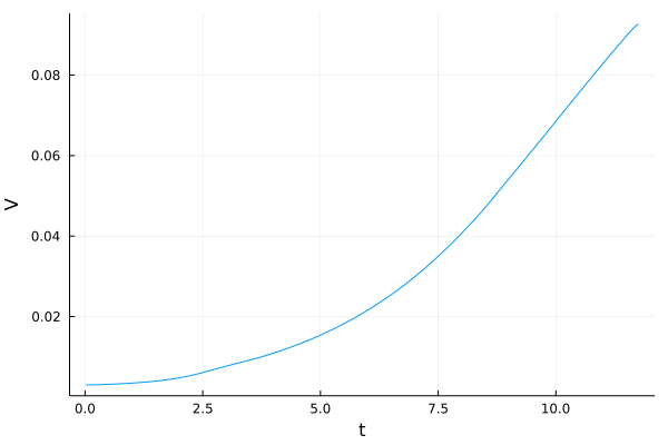
[23]:
deltat1 = value.(Δt)
t = (1:N)*deltat1[1]
s_plot = plot(t, s1, xlabel = "t", ylabel = "s", legend = false, fmt = :png)
p_plot = plot(t, p1, xlabel = "t", ylabel = "p", legend = false, fmt = :png)
r_plot = plot(t, r1, xlabel = "t", ylabel = "r", legend = false, fmt = :png)
V_plot = plot(t, V1, xlabel = "t", ylabel = "V", legend = false, fmt = :png)
u_plot = plot(t, u1, xlabel = "t", ylabel = "u", legend = false, fmt = :png)
display(plot(s_plot, p_plot, r_plot, u_plot, layout = (2, 2)))
display(plot(V_plot))

[24]:
function test(e)
# JuMP model, Ipopt solver
sys = Model(optimizer_with_attributes(Ipopt.Optimizer, "print_level" => 3))
set_optimizer_attribute(sys, "tol", 1e-9)
set_optimizer_attribute(sys, "max_iter", 1000)
# Parameters
# Giordano et al. (2015)
e_M = 3.6 # 1/h
k_R = 3.6 # 1/h
K_R = 1 # g/L
beta = 0.003 # L/g
# Yegorov et al. (2018)
k_X = 1 # 1/h
K_X = 1 # g/L
k_M = 4.32 #1.2*k_R
K_M = 33.33 #0.1/beta
K = beta*K_R
K_1 = beta*K_X
K_2 = beta*K_M
k_1 = k_X/k_R
k_2 = k_M/k_R
t0 = 0.0 # initial time
tf = 50 # final time
p0 = 0.003 # p0
r0 = 0.1 # r0
V0 = 0.003 # V0
s0=0.1
eta = e
Eps = s0+(p0+1)*V0
rmin = r0*(V0/Eps)
rmax = 1-(1-r0)*(V0/Eps)
N = 200 # grid size
JuMP.@variables(sys, begin
0. ≤ s[1:N] ≤ 1. # s
0. ≤ p[1:N] ≤ 1. # p
rmin ≤ r[1:N] ≤ rmax # r
0. ≤ V[1:N] ≤ eta*Eps # V
0. ≤ u[1:N] ≤ 1.
0. ≤ Δt[1] ≤ 1.
end)
# Objective
@objective(sys, Min, Δt[1])
# Initial conditions
@constraints(sys, begin
s[1] == s0
p[1] == p0
r[1] == r0
V[1] == V0
V[N] == eta*Eps
end)
# Dynamics, Crank-Nicolson scheme
@NLexpression(sys, wR[j = 1:N], p[j]/(K+p[j]))
@NLexpression(sys, wM[j = 1:N], k_2*s[j]/(K_2+s[j]))
for j in 1:N-1
@NLconstraint(sys, # s' = -wM*(1-r)*V
s[j+1] == s[j] + 0.5 * Δt[1] * (-wM[j]*(1-r[j])*V[j] - wM[j+1]*(1-r[j+1])*V[j+1]))
@NLconstraint(sys, # p' = wM*(1-r) - wR*r*(p+1)
p[j+1] == p[j] + 0.5 * Δt[1] * (wM[j]*(1-r[j]) - wR[j]*r[j]*(p[j]+1) + wM[j+1]*(1-r[j+1]) - wR[j+1]*r[j+1]*(p[j+1]+1)))
@NLconstraint(sys, # r' = (u-r)*wR*r
r[j+1] == r[j] + 0.5 * Δt[1] * ((u[j]-r[j])*wR[j]*r[j] + (u[j+1]-r[j+1])*wR[j+1]*r[j+1]))
@NLconstraint(sys, # v' = wR*r*V
V[j+1] == V[j] + 0.5 * Δt[1] * (wR[j]*r[j]*V[j] + wR[j+1]*r[j+1]*V[j+1]))
end
# Solve for the control and state
println("Solving...")
status = optimize!(sys)
println("Solver status: ", status)
deltat = value.(Δt)
println("Cost: ", objective_value(sys))
return deltat[1]*N
end
list_eta = [0.9, 0.91, 0.92, 0.93, 0.94, 0.95, 0.96, 0.97, 0.98, 0.99, 0.999]
list_tf = [0.,0.,0.,0.,0.,0.,0.,0.,0.,0.,0.]
list_rapport = [0.,0.,0.,0.,0.,0.,0.,0.,0.,0.,0.]
i=1
for e in list_eta
eta = e
tf = test(e)
list_tf[i] = tf
list_rapport[i] = e/tf
i=i+1
end
println(list_tf)
println(list_rapport)
Solving...
┌ Warning: Axis contains one element: 1. If intended, you can safely ignore this warning. To explicitly pass the axis with one element, pass `[1]` instead of `1`.
└ @ JuMP.Containers /Users/ocots/.julia/packages/JuMP/UqjgA/src/Containers/DenseAxisArray.jl:173
Total number of variables............................: 1001
variables with only lower bounds: 0
variables with lower and upper bounds: 1001
variables with only upper bounds: 0
Total number of equality constraints.................: 801
Total number of inequality constraints...............: 0
inequality constraints with only lower bounds: 0
inequality constraints with lower and upper bounds: 0
inequality constraints with only upper bounds: 0
Number of Iterations....: 283
(scaled) (unscaled)
Objective...............: 5.8941756157611581e-02 5.8941756157611581e-02
Dual infeasibility......: 8.4330601926219554e-14 8.4330601926219554e-14
Constraint violation....: 7.4843742314811834e-11 7.4843742314811834e-11
Variable bound violation: 0.0000000000000000e+00 0.0000000000000000e+00
Complementarity.........: 9.0909650918392711e-11 9.0909650918392711e-11
Overall NLP error.......: 9.0909650918392711e-11 9.0909650918392711e-11
Number of objective function evaluations = 299
Number of objective gradient evaluations = 284
Number of equality constraint evaluations = 299
Number of inequality constraint evaluations = 0
Number of equality constraint Jacobian evaluations = 284
Number of inequality constraint Jacobian evaluations = 0
Number of Lagrangian Hessian evaluations = 283
Total seconds in IPOPT = 3.619
EXIT: Optimal Solution Found.
Solver status: nothing
Cost: 0.05894175615761158
Solving...
┌ Warning: Axis contains one element: 1. If intended, you can safely ignore this warning. To explicitly pass the axis with one element, pass `[1]` instead of `1`.
└ @ JuMP.Containers /Users/ocots/.julia/packages/JuMP/UqjgA/src/Containers/DenseAxisArray.jl:173
Total number of variables............................: 1001
variables with only lower bounds: 0
variables with lower and upper bounds: 1001
variables with only upper bounds: 0
Total number of equality constraints.................: 801
Total number of inequality constraints...............: 0
inequality constraints with only lower bounds: 0
inequality constraints with lower and upper bounds: 0
inequality constraints with only upper bounds: 0
Number of Iterations....: 104
(scaled) (unscaled)
Objective...............: 5.9552845037091670e-02 5.9552845037091670e-02
Dual infeasibility......: 6.3289021342219113e-14 6.3289021342219113e-14
Constraint violation....: 5.6300075712556463e-11 5.6300075712556463e-11
Variable bound violation: 0.0000000000000000e+00 0.0000000000000000e+00
Complementarity.........: 9.0909686394900431e-11 9.0909686394900431e-11
Overall NLP error.......: 9.0909686394900431e-11 9.0909686394900431e-11
Number of objective function evaluations = 118
Number of objective gradient evaluations = 98
Number of equality constraint evaluations = 118
Number of inequality constraint evaluations = 0
Number of equality constraint Jacobian evaluations = 107
Number of inequality constraint Jacobian evaluations = 0
Number of Lagrangian Hessian evaluations = 104
Total seconds in IPOPT = 1.189
EXIT: Optimal Solution Found.
Solver status: nothing
Cost: 0.05955284503709167
Solving...
┌ Warning: Axis contains one element: 1. If intended, you can safely ignore this warning. To explicitly pass the axis with one element, pass `[1]` instead of `1`.
└ @ JuMP.Containers /Users/ocots/.julia/packages/JuMP/UqjgA/src/Containers/DenseAxisArray.jl:173
Total number of variables............................: 1001
variables with only lower bounds: 0
variables with lower and upper bounds: 1001
variables with only upper bounds: 0
Total number of equality constraints.................: 801
Total number of inequality constraints...............: 0
inequality constraints with only lower bounds: 0
inequality constraints with lower and upper bounds: 0
inequality constraints with only upper bounds: 0
Number of Iterations....: 106
(scaled) (unscaled)
Objective...............: 6.0220227957037291e-02 6.0220227957037291e-02
Dual infeasibility......: 1.3864999355506913e-14 1.3864999355506913e-14
Constraint violation....: 1.8253010214408505e-11 1.8253010214408505e-11
Variable bound violation: 0.0000000000000000e+00 0.0000000000000000e+00
Complementarity.........: 9.0909276302003908e-11 9.0909276302003908e-11
Overall NLP error.......: 9.0909276302003908e-11 9.0909276302003908e-11
Number of objective function evaluations = 118
Number of objective gradient evaluations = 100
Number of equality constraint evaluations = 118
Number of inequality constraint evaluations = 0
Number of equality constraint Jacobian evaluations = 109
Number of inequality constraint Jacobian evaluations = 0
Number of Lagrangian Hessian evaluations = 106
Total seconds in IPOPT = 1.190
EXIT: Optimal Solution Found.
Solver status: nothing
Cost: 0.06022022795703729
┌ Warning: Axis contains one element: 1. If intended, you can safely ignore this warning. To explicitly pass the axis with one element, pass `[1]` instead of `1`.
└ @ JuMP.Containers /Users/ocots/.julia/packages/JuMP/UqjgA/src/Containers/DenseAxisArray.jl:173
Solving...
Total number of variables............................: 1001
variables with only lower bounds: 0
variables with lower and upper bounds: 1001
variables with only upper bounds: 0
Total number of equality constraints.................: 801
Total number of inequality constraints...............: 0
inequality constraints with only lower bounds: 0
inequality constraints with lower and upper bounds: 0
inequality constraints with only upper bounds: 0
Number of Iterations....: 106
(scaled) (unscaled)
Objective...............: 6.0962196731351143e-02 6.0962196731351143e-02
Dual infeasibility......: 2.6157846118594333e-13 2.6157846118594333e-13
Constraint violation....: 1.3979539748021352e-10 1.3979539748021352e-10
Variable bound violation: 0.0000000000000000e+00 0.0000000000000000e+00
Complementarity.........: 9.0909819134957637e-11 9.0909819134957637e-11
Overall NLP error.......: 1.3979539748021352e-10 1.3979539748021352e-10
Number of objective function evaluations = 117
Number of objective gradient evaluations = 100
Number of equality constraint evaluations = 117
Number of inequality constraint evaluations = 0
Number of equality constraint Jacobian evaluations = 109
Number of inequality constraint Jacobian evaluations = 0
Number of Lagrangian Hessian evaluations = 106
Total seconds in IPOPT = 1.441
EXIT: Optimal Solution Found.
Solver status: nothing
Cost: 0.06096219673135114
Solving...
┌ Warning: Axis contains one element: 1. If intended, you can safely ignore this warning. To explicitly pass the axis with one element, pass `[1]` instead of `1`.
└ @ JuMP.Containers /Users/ocots/.julia/packages/JuMP/UqjgA/src/Containers/DenseAxisArray.jl:173
Total number of variables............................: 1001
variables with only lower bounds: 0
variables with lower and upper bounds: 1001
variables with only upper bounds: 0
Total number of equality constraints.................: 801
Total number of inequality constraints...............: 0
inequality constraints with only lower bounds: 0
inequality constraints with lower and upper bounds: 0
inequality constraints with only upper bounds: 0
Number of Iterations....: 112
(scaled) (unscaled)
Objective...............: 6.1800700228630261e-02 6.1800700228630261e-02
Dual infeasibility......: 1.6567566798854256e-13 1.6567566798854256e-13
Constraint violation....: 4.4287351563809807e-11 4.4287351563809807e-11
Variable bound violation: 0.0000000000000000e+00 0.0000000000000000e+00
Complementarity.........: 9.0909510325346938e-11 9.0909510325346938e-11
Overall NLP error.......: 9.0909510325346938e-11 9.0909510325346938e-11
Number of objective function evaluations = 128
Number of objective gradient evaluations = 106
Number of equality constraint evaluations = 128
Number of inequality constraint evaluations = 0
Number of equality constraint Jacobian evaluations = 115
Number of inequality constraint Jacobian evaluations = 0
Number of Lagrangian Hessian evaluations = 112
Total seconds in IPOPT = 1.434
EXIT: Optimal Solution Found.
Solver status: nothing
Cost: 0.06180070022863026
Solving...
┌ Warning: Axis contains one element: 1. If intended, you can safely ignore this warning. To explicitly pass the axis with one element, pass `[1]` instead of `1`.
└ @ JuMP.Containers /Users/ocots/.julia/packages/JuMP/UqjgA/src/Containers/DenseAxisArray.jl:173
Total number of variables............................: 1001
variables with only lower bounds: 0
variables with lower and upper bounds: 1001
variables with only upper bounds: 0
Total number of equality constraints.................: 801
Total number of inequality constraints...............: 0
inequality constraints with only lower bounds: 0
inequality constraints with lower and upper bounds: 0
inequality constraints with only upper bounds: 0
Number of Iterations....: 113
(scaled) (unscaled)
Objective...............: 6.2771790741277256e-02 6.2771790741277256e-02
Dual infeasibility......: 1.6402191683953715e-14 1.6402191683953715e-14
Constraint violation....: 1.0966394459188678e-11 1.0966394459188678e-11
Variable bound violation: 0.0000000000000000e+00 0.0000000000000000e+00
Complementarity.........: 9.0909191040505591e-11 9.0909191040505591e-11
Overall NLP error.......: 9.0909191040505591e-11 9.0909191040505591e-11
Number of objective function evaluations = 125
Number of objective gradient evaluations = 107
Number of equality constraint evaluations = 125
Number of inequality constraint evaluations = 0
Number of equality constraint Jacobian evaluations = 116
Number of inequality constraint Jacobian evaluations = 0
Number of Lagrangian Hessian evaluations = 113
Total seconds in IPOPT = 1.470
EXIT: Optimal Solution Found.
Solver status: nothing
Cost: 0.06277179074127726
Solving...
┌ Warning: Axis contains one element: 1. If intended, you can safely ignore this warning. To explicitly pass the axis with one element, pass `[1]` instead of `1`.
└ @ JuMP.Containers /Users/ocots/.julia/packages/JuMP/UqjgA/src/Containers/DenseAxisArray.jl:173
Total number of variables............................: 1001
variables with only lower bounds: 0
variables with lower and upper bounds: 1001
variables with only upper bounds: 0
Total number of equality constraints.................: 801
Total number of inequality constraints...............: 0
inequality constraints with only lower bounds: 0
inequality constraints with lower and upper bounds: 0
inequality constraints with only upper bounds: 0
Number of Iterations....: 115
(scaled) (unscaled)
Objective...............: 6.3933049470721162e-02 6.3933049470721162e-02
Dual infeasibility......: 3.4811652456819390e-14 3.4811652456819390e-14
Constraint violation....: 4.8635262483998076e-11 4.8635262483998076e-11
Variable bound violation: 0.0000000000000000e+00 0.0000000000000000e+00
Complementarity.........: 9.0909607788887396e-11 9.0909607788887396e-11
Overall NLP error.......: 9.0909607788887396e-11 9.0909607788887396e-11
Number of objective function evaluations = 135
Number of objective gradient evaluations = 109
Number of equality constraint evaluations = 135
Number of inequality constraint evaluations = 0
Number of equality constraint Jacobian evaluations = 118
Number of inequality constraint Jacobian evaluations = 0
Number of Lagrangian Hessian evaluations = 115
Total seconds in IPOPT = 1.312
EXIT: Optimal Solution Found.
Solver status: nothing
Cost: 0.06393304947072116
Solving...
┌ Warning: Axis contains one element: 1. If intended, you can safely ignore this warning. To explicitly pass the axis with one element, pass `[1]` instead of `1`.
└ @ JuMP.Containers /Users/ocots/.julia/packages/JuMP/UqjgA/src/Containers/DenseAxisArray.jl:173
Total number of variables............................: 1001
variables with only lower bounds: 0
variables with lower and upper bounds: 1001
variables with only upper bounds: 0
Total number of equality constraints.................: 801
Total number of inequality constraints...............: 0
inequality constraints with only lower bounds: 0
inequality constraints with lower and upper bounds: 0
inequality constraints with only upper bounds: 0
Number of Iterations....: 295
(scaled) (unscaled)
Objective...............: 6.5396669918009215e-02 6.5396669918009215e-02
Dual infeasibility......: 2.8171618595760094e-14 2.8171618595760094e-14
Constraint violation....: 1.5553280885427512e-11 1.5553280885427512e-11
Variable bound violation: 0.0000000000000000e+00 0.0000000000000000e+00
Complementarity.........: 9.0909258087795642e-11 9.0909258087795642e-11
Overall NLP error.......: 9.0909258087795642e-11 9.0909258087795642e-11
Number of objective function evaluations = 315
Number of objective gradient evaluations = 296
Number of equality constraint evaluations = 315
Number of inequality constraint evaluations = 0
Number of equality constraint Jacobian evaluations = 296
Number of inequality constraint Jacobian evaluations = 0
Number of Lagrangian Hessian evaluations = 295
Total seconds in IPOPT = 3.887
EXIT: Optimal Solution Found.
Solver status: nothing
Cost: 0.06539666991800921
Solving...
┌ Warning: Axis contains one element: 1. If intended, you can safely ignore this warning. To explicitly pass the axis with one element, pass `[1]` instead of `1`.
└ @ JuMP.Containers /Users/ocots/.julia/packages/JuMP/UqjgA/src/Containers/DenseAxisArray.jl:173
Total number of variables............................: 1001
variables with only lower bounds: 0
variables with lower and upper bounds: 1001
variables with only upper bounds: 0
Total number of equality constraints.................: 801
Total number of inequality constraints...............: 0
inequality constraints with only lower bounds: 0
inequality constraints with lower and upper bounds: 0
inequality constraints with only upper bounds: 0
Number of Iterations....: 323
(scaled) (unscaled)
Objective...............: 6.7412913476873837e-02 6.7412913476873837e-02
Dual infeasibility......: 9.2339857043987270e-14 9.2339857043987270e-14
Constraint violation....: 6.0219051967180803e-11 6.0219051967180803e-11
Variable bound violation: 0.0000000000000000e+00 0.0000000000000000e+00
Complementarity.........: 9.0909346900912258e-11 9.0909346900912258e-11
Overall NLP error.......: 9.0909346900912258e-11 9.0909346900912258e-11
Number of objective function evaluations = 385
Number of objective gradient evaluations = 321
Number of equality constraint evaluations = 385
Number of inequality constraint evaluations = 0
Number of equality constraint Jacobian evaluations = 325
Number of inequality constraint Jacobian evaluations = 0
Number of Lagrangian Hessian evaluations = 323
Total seconds in IPOPT = 4.002
EXIT: Optimal Solution Found.
Solver status: nothing
Cost: 0.06741291347687384
Solving...
┌ Warning: Axis contains one element: 1. If intended, you can safely ignore this warning. To explicitly pass the axis with one element, pass `[1]` instead of `1`.
└ @ JuMP.Containers /Users/ocots/.julia/packages/JuMP/UqjgA/src/Containers/DenseAxisArray.jl:173
Total number of variables............................: 1001
variables with only lower bounds: 0
variables with lower and upper bounds: 1001
variables with only upper bounds: 0
Total number of equality constraints.................: 801
Total number of inequality constraints...............: 0
inequality constraints with only lower bounds: 0
inequality constraints with lower and upper bounds: 0
inequality constraints with only upper bounds: 0
Number of Iterations....: 255
(scaled) (unscaled)
Objective...............: 7.0777073773047636e-02 7.0777073773047636e-02
Dual infeasibility......: 5.4835726278997076e-14 5.4835726278997076e-14
Constraint violation....: 1.6101286970382489e-11 1.6101286970382489e-11
Variable bound violation: 0.0000000000000000e+00 0.0000000000000000e+00
Complementarity.........: 9.0909224455371836e-11 9.0909224455371836e-11
Overall NLP error.......: 9.0909224455371836e-11 9.0909224455371836e-11
Number of objective function evaluations = 279
Number of objective gradient evaluations = 254
Number of equality constraint evaluations = 279
Number of inequality constraint evaluations = 0
Number of equality constraint Jacobian evaluations = 257
Number of inequality constraint Jacobian evaluations = 0
Number of Lagrangian Hessian evaluations = 255
Total seconds in IPOPT = 4.489
EXIT: Optimal Solution Found.
Solver status: nothing
Cost: 0.07077707377304764
Solving...
┌ Warning: Axis contains one element: 1. If intended, you can safely ignore this warning. To explicitly pass the axis with one element, pass `[1]` instead of `1`.
└ @ JuMP.Containers /Users/ocots/.julia/packages/JuMP/UqjgA/src/Containers/DenseAxisArray.jl:173
Total number of variables............................: 1001
variables with only lower bounds: 0
variables with lower and upper bounds: 1001
variables with only upper bounds: 0
Total number of equality constraints.................: 801
Total number of inequality constraints...............: 0
inequality constraints with only lower bounds: 0
inequality constraints with lower and upper bounds: 0
inequality constraints with only upper bounds: 0
Number of Iterations....: 476
(scaled) (unscaled)
Objective...............: 8.1638847117859986e-02 8.1638847117859986e-02
Dual infeasibility......: 9.2395503393960542e-14 9.2395503393960542e-14
Constraint violation....: 9.8965280415086454e-13 9.8965280415086454e-13
Variable bound violation: 0.0000000000000000e+00 0.0000000000000000e+00
Complementarity.........: 9.0909111959343482e-11 9.0909111959343482e-11
Overall NLP error.......: 9.0909111959343482e-11 9.0909111959343482e-11
Number of objective function evaluations = 766
Number of objective gradient evaluations = 465
Number of equality constraint evaluations = 766
Number of inequality constraint evaluations = 0
Number of equality constraint Jacobian evaluations = 480
Number of inequality constraint Jacobian evaluations = 0
Number of Lagrangian Hessian evaluations = 476
Total seconds in IPOPT = 9.948
EXIT: Optimal Solution Found.
Solver status: nothing
Cost: 0.08163884711785999
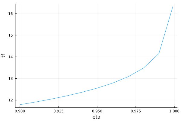
[11.788351231522316, 11.910569007418333, 12.044045591407459, 12.192439346270229, 12.360140045726052, 12.554358148255451, 12.786609894144233, 13.079333983601844, 13.482582695374767, 14.155414754609527, 16.327769423571997]
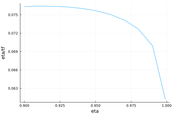
[0.07634655452014187, 0.0764027310058167, 0.07638629337772952, 0.07627677887809177, 0.07605091823575556, 0.07567093345445236, 0.07507853981215477, 0.07416279767885224, 0.07268637041893994, 0.0699379013022292, 0.06118410752161703]
Final time as a function of eta
[25]:
plot(list_eta, list_tf, xlabel = "eta", ylabel = "tf", legend = false, fmt = :png)
[25]:
[26]:
plot(list_eta, list_rapport, xlabel = "eta", ylabel = "eta/tf", legend = false, fmt = :png)
[26]:
[ ]: